A FLUKA beginner’s guide¶

Introduction¶

This Chapter is intended to provide a minimal set of instructions to install and run FLUKA for a beginner user, going through the different steps required to run a simple example. References to the relevant chapters of the manual are given to help the user in finding more detailed information on the different topics. After describing the installation procedure, instructions are given on how to build the input file for a simple case. Instructions for running and accessing the results are also reported. As a further step, the user is addressed to User routines to learn how to tailor FLUKA to specific needs by means of user routines.

Installing FLUKA¶

A full description of the installation procedure is given in Installation. The FLUKA packages are distributed as tar and RPM files which can be downloaded from the FLUKA website https://fluka.eu .

% mkdir fluka
% cd fluka
% tar zxvf ../fluka2011-linuxAA.tar.gz

% gunzip -dc ../fluka2011-linuxAA.tar.gz | tar xvf

% ...
% cd fluka
% export FLUPRO=$PWD

% ...
% cd fluka
% setenv FLUPRO $PWD

% cd \$FLUPRO
% \$FLUPRO/flutil/lfluka -m fluka

% make

Building a FLUKA input¶

Generalities about FLUKA input¶

FLUKA reads user input from an ASCII “standard input” file with extension .inp. The general characteristics and rules of FLUKA input are described in General features of FLUKA input. The input consists of a variable number of “commands” (called also “options”), each consisting of one or more “lines” (called also “cards” for historical reasons).

Apart from FLUKA commands, the input file may contain also the description of the geometry of the simulated set-up. Also this description is provided by means of specific geometry “command cards” in a special format described in Combinatorial Geometry.

The geometry description can, on request, be kept in a separate ASCII file: this feature is especially useful when the same geometry is used in several different inputs, not only to save space but because modifications can be made in one single place.

The typical structure of a FLUKA input file is the following:

Titles and comments for documentation purposes (optional, but recommended)
Description of the problem geometry (solid bodies and surfaces, combined to partition space into regions) (mandatory)
Definition of the materials (mandatory unless pre-defined materials are used)
Material assignments (correspondence material–region, mandatory)
Definition of the particle source (mandatory)
Definition of the requested “detectors”. Each of these is a phase space domain (region of space, particle direction and energy) where the user wants to calculate the expectation value of a physical quantity such as dose, fluence, etc. Various kinds of detectors are available, corresponding to different quantities and to different algorithms used to estimate them (“estimators”). Detectors are optional, but one at least is expected, at least in the production phase
Definition of biasing schemes (optional)
Definition of problem settings such as energy cutoffs, step size, physical effects not simulated by default, particles not to be transported, etc. (optional)
Initialisation of the random number sequence (mandatory if an estimation of the statistical error is desired)
Starting signal and number of requested histories (mandatory)

In addition, special commands are available in FLUKA for more advanced problems involving magnetic fields, time-dependent calculations, writing of history files (so-called “collision tapes”), transport of optical photons, event by event scoring, calling user-written routines, etc. These options are expected to be requested only by users having some previous experience with the more common commands: therefore they will be mostly ignored in this beginner’s guide.

Let’s first recall the general structure of the FLUKA command lines (cards). The geometry commands will be reviewed later. Each card contains:

one keyword,
six floating point values (called WHATs),
one character string (called SDUM)

Some WHATs represent numerical quantities (e.g. energy, coordinates), while others, converted to integers, are indices corresponding to a material, a type of particle, a region etc. In this latter case, it is possible to replace the number by the corresponding name (a character string).

Not necessarily all WHATs and SDUMs are used. In some cases, a command line can be followed by a line of text (for instance a filename path or a title). Any line having an asterisk (*) in the first position is treated as a comment. All lines (commands, text strings and comments) are echoed on the standard output (the file with extension .out). In case of problems, it is a good idea to check how every line has been printed in the standard output. Often, output reveals typing or format errors by showing how the program has misinterpreted them.

In addition to the simple echo, an “interpreted” feedback to all commands is provided in the next section of the standard output. Checking this part of the output is also very useful, because it helps making sure that the user’s intentions have been expressed correctly and understood by the code. See Output on FLUKA output for a detailed description.

If a line contains an exclamation mark (!) all following characters are replaced by blanks. This feature can be used for short in-line comments which will not be echoed in output.

The order of input commands is generally free, with only a few exceptions reported in General features of FLUKA input. Therefore, the order suggested in the following should not be considered as mandatory, but only one of the possible ways to write FLUKA input.

Input alignment¶

Be careful to properly align keywords and numbers. Format is not free, unless a command is issued at the beginning of input: see option GLOBAL in GLOBAL or FREE in FREE). Even in the free format for the input file, the part of the input describing the geometry can still be written in fixed format (which is different from the general FLUKA input format, see Combinatorial Geometry). There is the possibility of having free format also for the geometry part: this can also be activated using the GLOBAL command (see GLOBAL).

In fixed format, in order to ensure proper alignment, a comment line showing a scale can be used anywhere in the input file, for instance:

*...+....1....+....2....+....3....+....4....+....5....+....6....+....7....+....8

In numerical fields, blanks are treated as zero. Therefore, numbers written with a decimal period and without an exponent (e.g. 1.2345) can be placed anywhere inside their respective format fields. For instance, the following two input lines are equally acceptable:

BEAM      200.      0.2       1.5       1.2       0.7       1.0       PROTON
*...+....1....+....2....+....3....+....4....+....5....+....6....+....7....+....8
BEAM            200.       0.2       1.5       1.2       0.7       1.0PROTON

If a number is written in exponential notation (e.g. 2.3E5) or in integer form (without decimal point), it must be aligned to the right of the field. Depending on the platform and the compiler, sometimes the number is correctly interpreted even if the alignment rule is not respected. However this is not guaranteed and the right alignment rule should always be followed. For instance in:

*...+....1....+....2....+....3....+....4....+....5....+....6....+....7....+....8
BEAM          2.E2        0.2       1.5       1.2       0.7       1.  PROTON

the first value might be interpreted as 2.E200. Another case is the following:

*...+....1....+....2....+....3....+....4....+....5....+....6....+....7....+....8
BEAM      200.      0.2       1.5       1.2       0.7       1         PROTON

here the last numerical field would be interpreted as 1000000000. To avoid mistakes due to this kind of input errors, the present FLUKA versions now recognise such potential problems and the program is forced to stop. At the same time a message is printed on the standard output file, as shown here for the above example:

 *** The 6th field  1         of the following input card ***
BEAM      200.     0.2       1.5       1.2       0.7       1         PROTON
 *** does not contain a valid formatted fortran real number!!! ***
 *** It is ambiguous and it could be read differently on different compilers ***
 *** depending how strictly the blank=0 formatted input rule is implemented  ***

Keywords (character strings such as BEAM and PROTON) must be aligned to the left of their field and must be in upper case. An exception is the continuation character “ & ” used in some commands, which can be placed anywhere within its 10-characters field.

Non-numerical values of WHATs (“names”) can be aligned anywhere within the corresponding fixed-format fields.. Sometimes a special option requires a region or a particle number to be entered with a negative sign: in this case the equivalent name must also be entered preceded by a minus sign.

A simple example¶

Let us now consider a simple starting application. We want to calculate the charged pion fluence produced by a monochromatic proton beam of momentum 50 GeV/c impinging on a 5 cm thick beryllium target of simple shape: a small parallelepiped (20 cm $\times$ 20 cm $\times$ 5 cm). A further simplification will be made for the purpose of this example, neglecting all the surrounding environment and substituting it with ideal vacuum.

We will guide the reader through the different parts of a possible input file suited for this application. The information which follows is meant to serve as a guide, but does not cover all the important points. It is recommended that for each option card selected, the user read carefully the relevant manual entry, and especially the explanatory notes.

The title¶

Typically, an input file begins with a TITLE card followed by one line of text describing the problem, or identifying that particular run, or providing some kind of generic information. In our case, for example

*...+....1....+....2....+....3....+....4....+....5....+....6....+....7....+....8
TITLE
Charged pion fluence inside and around a proton-irradiated Be target

Further information can be provided by comment cards, but the title, because it is printed at the top of the standard output, is a useful reminder of what the corresponding file is about. In addition, the title is printed in all separate output files (error file, estimator files etc.) together with the date and time of the FLUKA run, allowing to keep track of their origin.

Commands such as GLOBAL and DEFAULTS, if needed, must immediately follow. Since this is intended as a beginner’s guide, these can be ignored here (for most common problems the defaults provided are sufficient). Let us recall that without specifying a DEFAULTS value, the NEW–DEFAults set of FLUKA parameters is loaded.

Definition of the primary particles¶

All “events” or “histories” are initiated by primary particles, which in the simplest case are monoenergetic, monodirectional and start from a single point in space (pencil beam). The card BEAM defines the particle energy (or momentum) while the card BEAMPOS controls their starting position and direction. These two commands can be used also to define particle beams having a simple angular or momentum distribution (Gaussian or rectangular) , or a simple transverse profile (Gaussian, rectangular or annular), or a simple space distribution of starting points (spherical, cartesian or cylindrical shell). Isotropic or semi-isotropic angular emission can be described as a special case of an angular rectangular distribution.

For particle sources with more complex distributions in energy, space and direction, the user must write, compile and link a special routine (SOURCE), following the instructions given in SOURCE: user-written source, and input a card SOURCE.

A summary of the input data concerning primary particles is printed in the standard output under the title “Beam properties”.

The beam definition for our example can be the following (monochromatic, monodirectional proton beam of momentum 50 GeV/c):

*...+....1....+....2....+....3....+....4....+....5....+....6....+....7....+....8
BEAM         50.E+00                                                  PROTON

In our example, the beam starting point is given by:

*...+....1....+....2....+....3....+....4....+....5....+....6....+....7....+....8
BEAMPOS          0.0       0.0     -50.0

In the cartesian geometry used by FLUKA, the previous card means that the beam is injected at x, y, z coordinates: 0, 0, -50 cm and is directed along the positive z axis. Of course, the choice of the point of injection, the direction, etc., must be coherent with the geometrical description of the set-up, as discussed in the following section.

The geometry¶

The input for the Combinatorial Geometry (bodies, regions and optional region volumes, see respectively Body types, Region data, Region Volumes) must be immediately preceded by a GEOBEGIN card (see GEOBEGIN and GEOBEGIN card) and immediately followed by a GEOEND card (see GEOEND and GEOEND card). These two cards follow the normal FLUKA format. It is recalled that the format for the geometry has its own special rules, described in Combinatorial Geometry.

Comment lines in the geometry input have an asterisk in first position as in the rest of FLUKA input (but on-line comments are not allowed). Body numerical data can be written in two different formats, a “short” one (field length 10) and a “long” one (field length 22). The latter one is to be preferred when higher precision is needed, for instance when using bodies such as truncated cones, cylinders or planes not aligned with axes. It must be realised that using too few decimals can cause geometry errors when bodies are combined into regions (portions of space not defined or doubly defined).

The whole geometry must be surrounded by a region of “blackhole” limited by a closed body (generally an RPP parallelepiped). It is often a good idea to make this body much larger than the minimum required size: this makes easier to introduce possible future extensions. In some cases, as in our basic example, it is also useful to surround the actual geometry by a region of ideal vacuum, and to have the blackhole region surrounding the vacuum. This can be useful, for instance, in order to start the trajectory of the primary particles outside the physical geometry (a particle may not be started on a boundary).

Both the body input section and the region input section must be ended with an END card (see Body END line and Region END line). Optionally, region volumes can be input between the region END card and the GEOEND card (this option can be requested by setting a special flag in the Geometry title card, see Geometry Title line). The only effect of specifying region volumes is to normalise per cm$^3$ the quantities calculated via the SCORE option (see below): for other estimators requiring volume normalisation the volume is input as part of the detector definition (USRTRACK, USRCOLL, USRYIELD), or is calculated directly by the program (USRBIN).

The GEOEND card indicates the end of the geometry description, but can also be used to invoke the geometry debugger.

The geometry output is an expanded echo of the corresponding input, containing information also on memory allocation and on the structure of composite regions made of several sub-regions by means of the OR operator.

A possible realisation of the geometry set up for our basic example can be seen in Fig. 2.1.

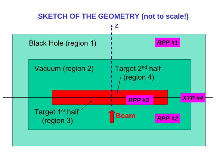
../_images/Geometry2.svg — Sketch of the geometry set–up of the example¶

Only four bodies are used here: an RPP body (Rectangular Parallelepiped, body no. 3, see Rectangular Parallelepiped. Code: RPP) to define a volume which will be the Be target region, inside another larger RPP body (no. 2), which will be filled with ideal vacuum and in turn is contained inside another larger RPP body (no. 1), to define the blackhole region. The fourth body, an XYP half-space (defined by a plane perpendicular to the z axis, see Infinite half-space delimited by a coordinate plane. Code: XYP, XZP, YZP), will be used to divide the target into 2 different regions: the upstream half will be defined as the portion of body 3 contained inside the half-space, and the downstream half as the portion outside it. Therefore, region “3” (the upstream half of the target) is the part of body no. 3 which is also inside body 4, while region “4” (downstream half of the target) is the part of body no. 3 which is not inside body 4. Region “2” (the vacuum around the target) is defined as the inside of body no. 2 from which body no. 3 is subtracted. Region “1” is simply the interior of body no. 1 from which body no. 2 is subtracted.

Note that bodies and regions can be identified by numbers, as described above, or with names (alphanumeric strings). The latter option is recommended, since it makes the preparation of the geometry much easier, especially if free format is also chosen. Here below we will show both possibilities.

The beam starting point has been chosen so that it is in the vacuum, outside the target region.

The geometry part of the input file can then be written as:

*...+....1....+....2....+....3....+....4....+....5....+....6....+....7....+....8
GEOBEGIN                                                              COMBINAT
    0    0               A simple Be target inside vacuum
  RPP    1-5000000.0+5000000.0-5000000.0+5000000.0-5000000.0+5000000.0
  RPP    2-1000000.0+1000000.0-1000000.0+1000000.0    -100.0+1000000.0
  RPP    3     -10.0     +10.0     -10.0     +10.0       0.0      +5.0
* plane to separate the upstream and downstream part of the target
  XYP    4       2.5
  END
* black hole
  BH1    5     +1     -2
* vacuum around
  VA2    5     +2     -3
* Be target 1st half
  BE3    5     +3     +4
* Be target 2nd half
  BE4    5     +3     -4
  END
GEOEND

The same geometry can be described in name-based free format as follows:

*...+....1....+....2....+....3....+....4....+....5....+....6....+....7....+....8
GEOBEGIN                                                              COMBNAME
    0    0               A simple Be target inside vacuum
  RPP blakhole -5000000.0  +5000000.0  -5000000.0  +5000000.0  -5000000.0  +5000000.0
  RPP vacumbox -1000000.0  +1000000.0  -1000000.0  +1000000.0      -100.0  +1000000.0
  RPP betarget      -10.0       +10.0       -10.0       +10.0         0.0        +5.0
* plane to separate the upstream and downstream part of the target
  XYP cutplane        2.5
  END
* black hole
  Blckhole  5  +blakhole -vacumbox
* vacuum around
  Vacarund  5  +vacumbox -betarget
* Be target 1st half
  UpstrBe   5  +betarget +cutplane
* Be target 2nd half
  DwnstrBe  5  +betarget -cutplane
  END
GEOEND

Materials¶

Each geometry region is supposed to be filled with a homogeneous material, or with vacuum, or with “blackhole”. The latter is a fictitious material used to terminate particle trajectories: any particle is discarded when reaching a blackhole boundary. Materials can be simple elements or compounds, where an element can have either natural composition or consist of a single nuclide, and compound indicates a chemical compound or a mixture or an alloy (or an isotopic mixture) of known composition.

An element can be either pre-defined (see list in Table 5.3 on page ) or defined by a MATERIAL card giving its atomic number, atomic weight, density, name and a material identification number > 2. The number of a non-pre-defined material can be chosen by the user, with the restriction that all lower numbers must also be defined (but not necessarily used). However, in a name-based input, it is convenient to leave the number blank: in this case the user does not need to know the number, which is assigned automatically by the code and will be used only internally.

Number 1 is reserved for blackhole and 2 for ideal vacuum. There are 25 pre-defined materials; but each of the numbers from 3 to 25 can be redefined, overriding the default definition. However, if the input is explicitly number-based only (via command GLOBAL), a pre-defined material can only be redefined using the same name by explicitly assigning to it a number equal to the original one . If the input is name-based, it is better to leave the number blank.

Materials can also be defined with higher index numbers, provided no gaps are left in the numbering sequence. For instance a material cannot be defined to have number 28 unless also 26 and 27 have been defined. Again, assigning explicitly a number is not necessary if the input is fully name-based.

A compound is defined by a MATERIAL card plus as many COMPOUND cards as needed to describe its composition. The MATERIAL card used to define a compound carries only the compound name, density and, if input is explicitly number-based only, material number (atomic number and atomic weight having no meaning in this case). Some special pre-defined compounds are available: for them the stopping power is not calculated by a formula but is determined using the parameters recommended by ICRU [ICRU84]. Reference to these pre-defined compounds is normally by name and no MATERIAL and COMPOUND cards are needed: if the input is explicitly number-based only (via command GLOBAL), a number needs to be assigned to them using a MATERIAL card, of course leaving no gaps in the numbering sequence.

Materials pre-defined or defined in the standard input are referred to as “FLUKA materials”, to distinguish them from materials available in the low-energy neutron cross section library (called “low-energy cross section materials”).

When transport of low-energy neutrons (E < 20 MeV) is requested (explicitly or by the chosen defaults), a correspondence is needed between each elemental (i.e. not compound) “FLUKA material” and one of the “low-energy cross section materials” available in the FLUKA low-energy neutron library. The default correspondence is set by the name and if more than one material with that name exist in the neutron library, the first in the list with that name (see 10.3) is assumed by default. The default can be changed using command LOW–MAT.

In the case of our example, only Beryllium is necessary, apart from blackhole and vacuum. In principle, since Beryllium is one of the pre-defined FLUKA materials, this part could even be omitted. However, for pedagogical reasons the following card is proposed, where index 5 is assigned to the target material:

*...+....1....+....2....+....3....+....4....+....5....+....6....+....7....+....8
MATERIAL         4.0       0.0     1.848       5.0                    BERYLLIU

Notice that the chosen name is BERYLLIU and not BERYLLIUM, in order to match the name in the list of “low-energy cross section materials” for low-energy neutrons (see Table 10.3), where material names have a maximum length of 8 characters.

The standard output concerning materials is very extended. First a list of multiple scattering parameters (printed by subroutine MULMIX) is reported for each material requested. This is mostly of scarce interest for the normal user, except for a table giving for each requested material the proportion of components, both by number of atoms (normalised to 1) and by weight (normalised to material density). The same information is repeated later on in another table entitled Material compositions.

If low-energy neutron transport has been requested (explicitly or by a chosen default), the following section reports the relevant material information: in particular, a table entitled “Fluka to low en. xsec material correspondence” specifies which material in the neutron cross section library has been mapped to each input material. Note that a much more detailed cross section information can be obtained by setting a printing flag (WHAT(4)) in the LOW–NEUT command.

The Table Material compositions contains information about the requested materials, those pre-defined by default and the elements used to define compounds. In addition to effective atomic number and atomic weight, density and composition, the table shows the value of some typical quantities: inelastic and elastic scattering length for the beam particles (not valid for electron and photon beams), radiation length and inelastic scattering length for 20 MeV neutrons.

The next table contains material data related to stopping power (average excitation energy, density effect parameters, and pressure in the case of gases) plus information about the implementation of various physical effects and the corresponding thresholds and tabulations.

The last material table is printed just before the beginning of the history calculations, and concerns the Correspondence of regions and EMF-FLUKA material numbers and names.

Assigning materials to regions¶

A material must be associated to each of the geometry regions, except to those defined as blackhole. This is done in a very straightforward way by command ASSIGNMAt. Assigning explicitly blackhole to a region is allowed, but is not necessary (except for region 2) because a region is blackhole by default unless another material has been associated to it. Region 2, if no material is assigned, is COPPER by default).

The table entitled Regions: materials and fields, in the standard output, can be consulted to check that material assignment has been done as desired.

For the present example the assignment could be:

*...+....1....+....2....+....3....+....4....+....5....+....6....+....7....+....8
*  Be target, 1st and 2nd half
ASSIGNMAT        5.0       3.0       4.0
*  External Black Hole
ASSIGNMAT        1.0       1.0
*  Vacuum
ASSIGNMAT        2.0       2.0

The same material assignments in a name-based input would be the following (BLCKHOLE and VACUUM are the pre-defined names of material 1 and 2):

*...+....1....+....2....+....3....+....4....+....5....+....6....+....7....+....8
*  Be target, 1st and 2nd half
ASSIGNMAT   BERYLLIU   UpstrBe  DwnstrBe
*  External Black Hole
ASSIGNMAT   BLCKHOLE  Blckhole
*  Vacuum
ASSIGNMAT     VACUUM  Vacarund

Production Thresholds¶

The implicit NEW–DEFA default setting, adopted in the example, sets, among other things, the production and transport threshold of heavy particles to 10 MeV. Production thresholds for $e^+$ $e^-$ and photons must be explicitly set using the EMFCUT command for all materials in the problem, as described in detail on. Let us choose also in this case a 10 MeV threshold for the single material of the example (previously marked with material index 5 and name BERYLLIU). Following the instructions about the EMFCUT option, the card can be written as:

*...+....1....+....2....+....3....+....4....+....5....+....6....+....7....+....8
EMFCUT        -0.010     0.010       1.0       5.0                    PROD-CUT

where the first numerical field is the threshold for $e^+$ $e^-$ (the minus sign meaning kinetic energy) and the second is for photons. The material number is given in the fourth numerical field. For details on all other parameters, and for other possibilities (for example how to introduce a transport cutoff different from production threshold) the user must accurately consult the Notes in EMFCUT.

In a name-based input, the above card could be:

*...+....1....+....2....+....3....+....4....+....5....+....6....+....7....+....8
EMFCUT        -0.010     0.010       1.0  BERYLLIU                    PROD-CUT

Production and transport threshold for all other particles can be overwritten using the PART–THRes command .

Estimators and Detectors¶

Even though, for setting-up purposes, it is conceivable that no detector be requested in a preliminary run, in most cases FLUKA is used to predict the expectation value of one or more quantities, as determined by the radiation field and by the material geometry described by the user: for such a task several different estimators are available. The quantities which are most commonly scored are dose and fluence, but others are available. Dose equivalent is generally calculated from differential fluence using conversion coefficients.

The simplest estimator available to the user is a historical vestige, survived from the “ancient” FLUKA (pre-1988) where the only possible output quantities were energy deposition and star density in regions. It is invoked by option SCORE, requesting evaluation of one to four different quantities. These can be different forms of energy density (proportional to dose), or of star density (approximately proportional to fluence of selected high-energy hadrons).

For this estimator, the detectors are pre-determined: the selected quantities are reported for each region of the geometry. The corresponding results, printed in the main output immediately after the last history has been completed, are presented in 6 columns as follows:

region  region   region     first       second      third       fourth
number   name    volume    quantity    quantity    quantity    quantity
  1     ......   ......    ........    ........    ........    ........
  2     ......   ......    ........    ........    ........    ........

etc.

on a line for each geometry region. The region volumes (in cm$^3$) have the value 1.0, or values optionally supplied by the user at the end of the geometry description (see Geometry Title line). All other columns are normalised per region volume and per primary particle.

The input could be as follows:

*...+....1....+....2....+....3....+....4....+....5....+....6....+....7....+....8
* score in each region energy deposition and stars produced by primaries
SCORE          208.0     210.0

The same, in a name-based input:

*...+....1....+....2....+....3....+....4....+....5....+....6....+....7....+....8
SCORE         ENERGY  BEAMPART

Other estimators are more flexible: the corresponding detectors can be requested practically in any number, can be written as unformatted or text files, and in most cases can provide differential distributions with respect to one or more variables. On the other hand, their output is presented in a very compact array form and must generally be post-processed by the user. For this purpose several utility programs are available: but output in text format can even be exported to a spreadsheet for post-processing.

USRBDX is the command required to define a detector for the boundary-crossing estimator. It calculates fluence or current, mono- or bi-directional, differential in energy and angle on any boundary between two selected regions. The area normalisation needed to obtain a current in particles per cm$^2$ is performed using an area value input by the user: if none is given, the area is assumed to be = 1.0 cm$^2$ and the option amounts simply to counting the total number of particles crossing the boundary. Similarly if fluence is scored, but in this case each particle is weighted with the secant of the angle between the particle trajectory and the normal to the boundary surface at the crossing point.

This is one of the estimators proposed for our example. We will request two boundary crossing detectors, one to estimate fluence and one for current, of particles crossing the boundary which separates the upstream and the downstream half of the target.

The following group of cards can be inserted:

*...+....1....+....2....+....3....+....4....+....5....+....6....+....7....+....8
* Boundary crossing fluence in the middle of the target (log intervals, one-way)
USRBDX          99.0     209.0     -47.0       3.0       4.0     400. piFluenUD
USRBDX         +50.0               +50.0                 0.0      10.0 &
*
* Boundary crossing current in the middle of the target (log intervals, one-way)
USRBDX          -1.0     209.0     -47.0       3.0       4.0     400. piCurrUD
USRBDX        +50.00               +50.0                 0.0      10.0 &

The same, in a name-based input:

*...+....1....+....2....+....3....+....4....+....5....+....6....+....7....+....8
USRBDX          99.0   PIONS+-     -47.0   UpstrBe  DwnstrBe     400. piFluenUD
USRBDX         +50.0               +50.0                 0.0      10.0 &
*
USRBDX          -1.0   PIONS+-     -47.0   UpstrBe  DwnstrBe     400. piCurrUD
USRBDX        +50.00               +50.0                 0.0      10.0 &

According to the instructions reported in USRBDX, it can be seen that the combined fluence of $\pi^+$ and $\pi^-$ is requested only when particles exit region “3” (“UpstrBe”, the upstream half of the target) to enter into region “4” (“DwnstrBe”, the downstream half). There is no interest in the reverse, therefore “one-way scoring” is selected. The scoring of the first detector will be inverse cosine-weighted, in order to define correctly the fluence. Results will be written unformatted on unit 47 for both quantities (so there will be two “Detectors” on the same output unit, but this is not mandatory). The energy distribution is going to be binned in 50 logarithmic intervals, from 0.001 GeV (the default minimum) up to 50 GeV. The angular distribution will be binned into 10 linear solid angle intervals from 0. to 2$\pi$ (having chosen the one-way estimator). The results will be normalised dividing by the area of the boundary (separation surface between the two regions, in this case the transverse section of the target), and will provide a double-differential fluence or current averaged over that surface (in cm$^{-2}$ GeV$^{-1}$ sr$^{-1}$).

Other fluence scoring options, based respectively on a track-length and on a collision estimator, are USRTRACK and USRCOLL which request the estimation of volume-averaged fluence (differential in energy) for any type of particle or family of particles in any selected region. The volume normalisation needed to obtain the fluence as track-length density or collision density is performed using a volume value input by the user: if none is given, the volume is assumed to be = 1.0 cm$^3$ and the result will be respectively the total track-length in that region, or the total number of collisions (weighted with the mean free path at each collision point).

Note that if additional normalisation factors are desired (e.g. beam power), this can be achieved by giving in input the “volume” or “area” value multiplied or divided by those factors. Options USRTRACK, USRCOLL and USRBDX can also calculate energy fluence, if the “particle” type is set = 208.0 (energy, name ENERGY) or 211.0 (electron and photon energy, name EM-ENRGY).

In our example, we are requesting two track-length detectors, to get the average fluence in the upstream half and in the downstream half of the target, respectively.

*...+....1....+....2....+....3....+....4....+....5....+....6....+....7....+....8
* Track-length fluence inside the target, Upstream part and Downstream part
* Logarithmic energy intervals
USRTRACK        -1.0     209.0     -48.0       3.0    1000.0      20. piFluenU
USRTRACK        50.0     0.001                                           &
USRTRACK        -1.0     209.0     -49.0       4.0    1000.0      20. piFluenD
USRTRACK        50.0     0.001                                           &

The volume input is $20 \times 20 \times 2.5 = 1000$ cm$^3$. We are requesting an energy spectrum in 20 logarithmic intervals between 0.001 and 50 GeV. In this case, we ask that the corresponding output be printed, unformatted, on two different files.

In a name-based input, the above example could be:

*...+....1....+....2....+....3....+....4....+....5....+....6....+....7....+....8
USRTRACK        -1.0   PIONS+-     -48.0   UpstrBe    1000.0      20. piFluenU
USRTRACK        50.0     0.001                                           &
USRTRACK        -1.0   PIONS+-     -49.0  DwnstrBe    1000.0      20. piFluenD
USRTRACK        50.0     0.001                                           &

Option USRBIN provides detailed space distributions of energy deposition, star density or integrated fluence (not energy fluence, unless by writing a special user routine). Using some suitable graphics package, USRBIN output can be presented in the form of colour maps. Programs for this purpose are available in the $FLUPRO/flutil directory (Pawlevbin.f and various kumac files), and on the FLUKA website www.fluka.eu.

USRBIN results are normalised to bin volumes calculated automatically by the program (except in the case of region binning and special 3-variable binning which are only seldom used).

The binning structure does not need to coincide with any geometry region. In our example we propose to ask for two Cartesian space distributions, one of charged pion fluence and one of total energy deposited. The first will extend over a volume larger than the target, because fluence can be calculated even in vacuum. Energy deposition, on the other hand, will be limited to the target volume.

*...+....1....+....2....+....3....+....4....+....5....+....6....+....7....+....8
* Cartesian binning of the pion fluence inside and around the target
USRBIN          10.0     209.0     -50.0      50.0      50.0      50. piFluBin
USRBIN         -50.0     -50.0     -10.0     100.0     100.0      60.0   &
* Cartesian binning of the deposited energy inside the target
USRBIN          10.0     208.0     -51.0      10.0      10.0       5. Edeposit
USRBIN         -10.0     -10.0       0.0      20.0      20.0       5.0   &

Also in this case, the request is for output on two separate files.

Or, using names:

*...+....1....+....2....+....3....+....4....+....5....+....6....+....7....+....8
USRBIN          10.0   PIONS+-     -50.0      50.0      50.0      50. piFluBin
USRBIN         -50.0     -50.0     -10.0     100.0     100.0      60.0   &
USRBIN          10.0    ENERGY     -51.0      10.0      10.0       5. Edeposit
USRBIN         -10.0     -10.0       0.0      20.0      20.0       5.0   &

Angular yields around a fixed direction of particles exiting a given surface can be calculated using option USRYIELD. The results are double-differential distributions with respect to a pair of variables, one of which is generally energy-like (kinetic energy, momentum, etc.) and the other one angle-like (polar angle, rapidity, Feynman-x, etc.) Distributions in LET (Linear Energy Transfer) can also be requested by this option. An arbitrary normalisation factor can be input.

Another commonly used scoring option is RESNUCLEi , which calculates residual nuclei production in a given region. A normalisation factor (usually the region volume) can be input.

A detailed summary of the requested detectors is printed on standard output. The same information is printed in the same format in estimator ASCII output files, and is available in coded form in estimator unformatted output files.

Initialisation of the random number sequence¶

The random number sequence used in a run is initialised by default by the seeds contained in file random.dat provided with the code. To calculate the statistical error of the results, it is necessary to perform other independent runs (at least 4 or 5), each with a different independent initialisation, using the seeds written by the program at the end of each run. The rfluka script provided with the code on UNIX and LINUX platforms takes care of this task, provided the following card is issued in the input file:

*...+....1....+....2....+....3....+....4....+....5....+....6....+....7....+....8
RANDOMIZe        1.0       0.0

The seeds of the random number generator are printed on a special file in hexadecimal form at the end of each group of histories (the size of a group depends on the number of histories requested in the START card).

Instead of getting the seeds from the last run, it is also possible to initialise directly another independent random number sequence by setting the second RANDOMIZE parameter equal to a different number, for instance:

*...+....1....+....2....+....3....+....4....+....5....+....6....+....7....+....8
RANDOMIZE        1.0     1198.

Starting signal and number of requested histories¶

At the end of the input file, a START card is mandatory in order to actually start the calculation. That card must indicate also the number of particle histories requested. The run, however, may be completed before all the histories have been handled in two cases: if a time limit has been met (on some systems) or if a “stop file” is created by the user (see instructions in Note 2 to option START).

The START card is optionally followed by a STOP card. For example, if the user wants to generate 100000 histories, the input file can be closed with the following two cards:

*...+....1....+....2....+....3....+....4....+....5....+....6....+....7....+....8
START       100000.0
STOP

The sample input file¶

In summary, the input file for our basic example (example.inp) name-based and written in fixed format, could be the following:

*...+....1....+....2....+....3....+....4....+....5....+....6....+....7....+....8
TITLE
Charged pion fluence inside and around a proton-irradiated Be target
*...+....1....+....2....+....3....+....4....+....5....+....6....+....7....+....8
BEAM         50.E+00                                                  PROTON
BEAMPOS          0.0       0.0     -50.0
*
 GEOBEGIN                                                              COMBNAME
                         A simple Be target inside vacuum
  RPP blakhole -5000000.0  +5000000.0  -5000000.0  +5000000.0  -5000000.0  +5000000.0
  RPP vacumbox -1000000.0  +1000000.0  -1000000.0  +1000000.0      -100.0  +1000000.0
  RPP betarget      -10.0       +10.0       -10.0       +10.0         0.0        +5.0
* plane to separate the upstream and downstream part of the target
  XYP cutplane        2.5
  END
* black hole
  Blckhole  5  +blakhole -vacumbox
* vacuum around
  Vacarund  5  +vacumbox -betarget
* Be target 1st half
  UpstrBe   5  +betarget +cutplane
* Be target 2nd half
  DwnstrBe  5  +betarget -cutplane
  END
GEOEND
*...+....1....+....2....+....3....+....4....+....5....+....6....+....7....+....8
MATERIAL         4.0       0.0     1.848       5.0                    BERYLLIU
*...+....1....+....2....+....3....+....4....+....5....+....6....+....7....+....8
*  Be target, 1st and 2nd half
ASSIGNMAT   BERYLLIU   UpstrBe  DwnstrBe
*  External Black Hole
ASSIGNMAT   BLCKHOLE  Blckhole
*  Vacuum
ASSIGNMAT     VACUUM  Vacarund
*...+....1....+....2....+....3....+....4....+....5....+....6....+....7....+....8
* e+e- and gamma production threshold set at 10 MeV
EMFCUT        -0.010     0.010       1.0  BERYLLIU                    PROD-CUT
* score in each region energy deposition and stars produced by primaries
SCORE         ENERGY  BEAMPART
* Boundary crossing fluence in the middle of the target (log intervals, one-way)
USRBDX          99.0   PIONS+-     -47.0   UpstrBe  DwnstrBe     400. piFluenUD
USRBDX         +50.0               +50.0                 0.0      10.0 &
* Boundary crossing current in the middle of the target (log intervals, one-way)
USRBDX          -1.0   PIONS+-     -47.0   UpstrBe  DwnstrBe     400. piCurrUD
USRBDX        +50.00               +50.0                 0.0      10.0 &
* Tracklength fluence inside the target, Upstream part and Downstream part
* Logarithmic energy intervals
USRTRACK        -1.0   PIONS+-     -48.0   UpstrBe    1000.0      20. piFluenU
USRTRACK        50.0     0.001                                           &
USRTRACK        -1.0   PIONS+-     -49.0  DwnstrBe    1000.0      20. piFluenD
USRTRACK        50.0     0.001                                           &
* Cartesian binning of the pion fluence inside and around the target
USRBIN          10.0   PIONS+-     -50.0      50.0      50.0      50. piFluBin
USRBIN         -50.0     -50.0     -10.0     100.0     100.0      60.0   &
* Cartesian binning of the deposited energy inside the target
USRBIN          10.0    ENERGY     -51.0      10.0      10.0       5. Edeposit
USRBIN         -10.0     -10.0       0.0      20.0      20.0       5.0   &
*...+....1....+....2....+....3....+....4....+....5....+....6....+....7....+....8
RANDOMIZe        1.0
*...+....1....+....2....+....3....+....4....+....5....+....6....+....7....+....8
START       100000.0
STOP

The same input file, number-based and using the free format option for the FLUKA commands, but not for the geometry, can instead be written as follows:

*...+....1....+....2....+....3....+....4....+....5....+....6....+....7....+....8
TITLE
Charged pion fluence inside and around a proton-irradiated Be target
*...+....1....+....2....+....3....+....4....+....5....+....6....+....7....+....8
GLOBAL                                         2.0
BEAM  50.E+00 0. 0. 0. 0. 0. PROTON
BEAMPOS  0. 0. -50.0 0. 0. 0. ' '
*...+....1....+....2....+....3....+....4....+....5....+....6....+....7....+....8
GEOBEGIN                                                              COMBINAT
                         A simple Be target inside vacuum
  RPP    1-5000000.0+5000000.0-5000000.0+5000000.0-5000000.0+5000000.0
  RPP    2-1000000.0+1000000.0-1000000.0+1000000.0    -100.0+1000000.0
  RPP    3     -10.0     +10.0     -10.0     +10.0       0.0      +5.0
  XYP    4       2.5
  END
* black hole
  BH1    5     +1     -2
* vacuum around
  VA2    5     +2     -3
* Be target 1st half
  BE3    5     +3     +4
* Be target 2nd half
  BE4    5     +3     -4
  END
GEOEND
MATERIAL  4.0 9.0122 1.848 5.0 0. 0. BERYLLIU
*  Be target, 1st and 2nd half
ASSIGNMAT 5.0 3.0 4.0 0. 0. 0.
*  External Black Hole
ASSIGNMAT 1.0 1.0 0. 0. 0. 0.
*  Vacuum
ASSIGNMAT 2.0 2.0 0. 0. 0. 0.
* e+e- and gamma production threshold set at 10 MeV
EMFCUT -0.010 0.010 1.0 5.0, , , PROD-CUT
* score in each region energy deposition and stars produced by primaries
SCORE 208.0 210. 0. 0. 0. 0.
* Boundary crossing fluence in the middle of the target (log intervals, one-way)
USRBDX  99.0 +209.0 -47.0 3.0 4.0 +400.0 piFluenUD
USRBDX  +50.00 0. +50.0 0. 0. 10.0 &
* Boundary crossing current in the middle of the target (log intervals, one-way)
USRBDX  -1.0 +209.0 -47.0 3.0 4.0 +400.0 piCurrUD
USRBDX  +50.00 0. +50.0 0. 0. 10.0 &
* Tracklength fluence inside the target, Upstream part and Downstream part
* Logarithmic energy intervals
USRTRACK -1.0 209.0 -48.0 3.0 1000.0 20. piFluenU
USRTRACK 50.0 0.001  0. 0. 0. 0. &
USRTRACK -1.0 209.0 -49.0 4.0 1000.0 20. piFluenD
USRTRACK 50.0 0.001  0. 0. 0. 0. &
* Cartesian binning of the pion fluence inside and around the target
USRBIN  10.0 209.0 -50.0  50.0  50.0  50. piFluBin
USRBIN  -50.0 -50.0 -10.0 100.0 100.0 60.0 &
* Cartesian binning of the deposited energy inside the target
USRBIN  10.0 208.0 -51.0 10.0 10.0 5. Edeposit
USRBIN  -10.0 -10.0 0.0 20.0 20.0 5.0 &
RANDOMIZe 1.0 0. 0. 0. 0. 0.
START  100000.0 0. 0. 0. 0. 0.
STOP

Other possible combinations are name-based free format and number-based fixed format.

Running FLUKA¶

It is advisable, but not mandatory, to keep separate the $FLUPRO directory from that or those where calculations are run and input files are kept. For instance, flukawork:

cd /home/user/flukawork

As mentioned above, the rfluka script in $FLUPRO/flutil should be used to drive the FLUKA run. In the following it is supposed that the user is going to ask for five statistically independent runs, each one made of 100000 histories, of the proposed basic example. The command is:

\$FLUPRO/flutil/rfluka -N0 -M5 example &

(on LINUX/UNIX, the & character allows to run the program in the background without “freezing” the terminal window).

The script creates a temporary subdirectory called fluka_nnnn where nnnn is the number of the subprocess. For instance, when the first run (or “cycle”) starts, the user will see on the terminal lines similar to the following ones:

$TARGET_MACHINE = Linux
$FLUPRO = /home/user/flupro
2789: old priority 0, new priority 10

Initial seed already existing

Running fluka in /home/user/flukawork/fluka_2789

================================ Running FLUKA for cycle # 1 ============================

At the end of each cycle the output files will be copied onto the running directory, the temporary directory will be erased and a new one will be created where the next run will take place. The names of the output files from each run are built by appending to the input file name the run number and an extension depending on their content: .out for the standard output, .err for the error file, .log for the log file and _fort.nn for the estimator files (with nn = absolute value of the selected output unit). The file containing the random number seeds will be called ran$<$input file name$><$run number$>$.

The error file may contain error messages related to the event generators (for instance when the program does not manage to conserve exactly energy or another quantity) or to the geometry tracking. Most of those are generally only warning messages which can be ignored unless there is a large number of them.

The log file generally contains messages related to fatal errors (input errors, overflow, etc.)

During a multiple run, lines like the following will appear on the user’s screen:

================================ Running FLUKA for cycle # 1 ====================

Removing links

Removing temporary files

Saving output and random number seed

Saving additional files generated
     Moving fort.47 to /home/fasso/Fluka/test/example01_fort.47
     Moving fort.48 to /home/fasso/Fluka/test/example01_fort.48
     Moving fort.49 to /home/fasso/Fluka/test/example01_fort.49
     Moving fort.50 to /home/fasso/Fluka/test/example01_fort.50
     Moving fort.51 to /home/fasso/Fluka/test/example01_fort.51

================================ Running FLUKA for cyle # 2 ====================

Removing links

Removing temporary files

Saving output and random number seed

Saving additional files generated
     Moving fort.47 to /home/fasso/Fluka/test/example002_fort.47
     Moving fort.48 to /home/fasso/Fluka/test/example002_fort.48
     Moving fort.49 to /home/fasso/Fluka/test/example002_fort.49
     Moving fort.50 to /home/fasso/Fluka/test/example002_fort.50
     Moving fort.51 to /home/fasso/Fluka/test/example002_fort.51

================================ Running FLUKA for cycle # 3 ===================

.....

================================ Running FLUKA for cycle # 4 ===================

.....

================================ Running FLUKA for cycle # 5 ===================

Removing links

Removing temporary files

Saving output and random number seed

Saving additional files generated
    Moving fort.47 to /home/fasso/Fluka/test/example005_fort.47
    Moving fort.48 to /home/fasso/Fluka/test/example005_fort.48
    Moving fort.49 to /home/fasso/Fluka/test/example005_fort.49
    Moving fort.50 to /home/fasso/Fluka/test/example005_fort.50
    Moving fort.51 to /home/fasso/Fluka/test/example005_fort.51

End of FLUKA run

At this time, in the working directory, the following new files exist:

example001_fort.47   example002_fort.47   ....   example005_fort.47
example001_fort.48   example002_fort.48   ....   example005_fort.48
example001_fort.49   example002_fort.49   ....   example005_fort.49
example001_fort.50   example002_fort.50   ....   example005_fort.50
example001_fort.51   example002_fort.51   ....   example005_fort.51
example001.out       example002.out       ....   example005.out
example001.err       example002.err       ....   example005.err

In Output the user can find a comprehensive description of the content of the FLUKA standard output. For the purpose of this beginner’s guide, it can just be pointed out that, according to the content of the USRBDX command, the files with extension fort.47 contain, in binary form, the boundary crossing estimator output for the required pion fluence and current detectors (for more details see USRBDX output). These files must be combined together to produce a table of values with their statistical errors which can be easily interfaced by the user to some analysis codes and/or graphic visualisation tools. Similarly, the files with extension fort.48 and fort.49 will contain the track-length estimator output, and those with extension fort.50 and fort.51 the output from USRBIN.

Accessing results¶

Boundary crossing estimator¶

Binary files from the USRBDX estimator can be accessed by means of the Usxsuw.f readout code, which is located in the $FLUPRO/flutil directory.

That readout code can be easily compiled. For example, the same compiling and linking FLUKA tools can be used for this purpose:

cd \$FLUPRO/flutil
./lfluka usxsuw.f -o usxsuw

The simplest way, however, is to use the makefile​ which is available in the $FLUPRO/flutil directory. In that directory, just type:
make
and all the post-processing utilities will be compiled and linked.

In order to process the 5 output files produced by the proposed example, the following interactive procedure can be used:

cd /home/user/flukawork
\$FLUPRO/flutil/usxsuw

The readout code will ask for the first FLUKA detector file name:

Type the input file:

For each detector file the program will show the content of the TITLE card of the FLUKA input file, the date and time of the FLUKA run and the number of histories for the given run.

The request will be iterated until a blank line is given. This will be interpreted as the end of the list of files, and then a name for the output file prefix will be requested. Let’s use, for example, the prefix pionbdx:

Type the input file: example001_fort.47
Charged pion fluence inside and around a proton-irradiated Be target
DATE:  7/15/ 5,  TIME: 16:22:11
 100000.
100000
Type the input file: example002_fort.47
Charged pion fluence inside and around a proton-irradiated Be target
DATE:  7/15/ 5,  TIME: 16:23: 3
 100000.
100000
Type the input file: example003_fort.47
Charged pion fluence inside and around a proton-irradiated Be target
DATE:  7/15/ 5,  TIME: 16:23:54
 100000.
100000
Type the input file: example004_fort.47
Charged pion fluence inside and around a proton-irradiated Be target
DATE:  7/15/ 5,  TIME: 16:24:51
 100000.
100000
Type the input file: example005_fort.47
Charged pion fluence inside and around a proton-irradiated Be target
DATE:  7/15/ 5,  TIME: 16:25:45
 100000.
100000
Type the input file: \
Type the output file name: pionbdx

At this point the following 3 new files are produced:

pionbdx
piobdxn_sum.lis
pionbdx_tab.lis

The first one (pionbdx) is again a binary file that can be read out at any time by Usxsuw. The content of this file is statistically equivalent to that of the sum of the files used to obtain it, and it can replace them to be combined with further output files if desired (the Usxsuw program takes care of giving it the appropriate weight). The other two files are ASCII text files.

Let us first examine pionbdx_sum.lis. This contains many comments which can help the user to understand the results. Since by means of the USRBDX command separate detectors for pion fluence and current have been requested, with their output on the same logical unit, there will be two different sections in the file, identified by the word “Detector”: Detector no. 1 is for fluence and Detector no. 2 is for current, because this is the order in which the USRBDX commands have been given.

Let us inspect the output from Detector no. 1:

Charged pion fluence inside and around a proton-irradiated Be target

  Total primaries run: 500000
  Total weight of the primaries run:  500000.

 Detector n:  1( 1)  piFluenUD
    (Area:         400. cmq,
     distr. scored: 209   ,
     from reg. 3 to  4,
     one way scoring,
     fluence scoring)

    Tot. resp. (Part/cmq/pr)  8.6904905E-04  +/-  0.6976866     %
    ( -->      (Part/pr)      0.3476196      +/-  0.6976866     % )

The total (summed) number of primaries (histories) is reported at first, then the main features of USRBDX request are summarised. The following numbers represent the energy and angle integrated fluence (“total response”).

Here and later, the statistical error is always expressed in percentage.

After this heading, the differential fluence tabulation as a function of (pion) energy, and integrated over solid angle, is reported, starting with the boundaries of the energy bins. As a general convention, these values are given from the highest to the lowest value:

**** Different. Fluxes as a function of energy ****
****      (integrated over solid angle)        ****

Energy boundaries (GeV):

99992       40.27077       32.43475       26.12349       21.04029
94620       13.64875       10.99293       8.853892       7.131072
743484       4.625898       3.725775       3.000802       2.416896
946608       1.567831       1.262757       1.017045      0.8191454
6597533      0.5313764      0.4279793      0.3447017      0.2776285
2236066      0.1800965      0.1450527      0.1168279      9.4095118E-02
5785778E-02  6.1039131E-02  4.9161937E-02  3.9595842E-02  3.1891152E-02
5685664E-02  2.0687662E-02  1.6662188E-02  1.3420003E-02  1.0808695E-02
7055033E-03  7.0115575E-03  5.6472253E-03  4.5483690E-03  3.6633324E-03
9505091E-03  2.3763892E-03  1.9139835E-03  1.5415541E-03  1.2415934E-03
Lowest boundary   (GeV):  1.0000000E-03

Flux (Part/GeV/cmq/pr):

5418744E-09 +/-    99.00000     %   4.8503271E-08 +/-    6.709127     %
3456116E-07 +/-    6.506497     %   5.9040013E-07 +/-    3.466331     %
2585346E-06 +/-    4.051404     %   2.5295039E-06 +/-    2.039807     %
6113087E-06 +/-    2.195296     %   7.6260553E-06 +/-    1.939942     %
2214471E-05 +/-   0.8310503     %   1.8394410E-05 +/-   0.6178440     %
6636921E-05 +/-    1.128397     %   3.6855919E-05 +/-    1.204921     %
1703457E-05 +/-    1.100655     %   6.9101960E-05 +/-   0.7564522     %
0419722E-05 +/-    1.799108     %   1.1945122E-04 +/-    1.256268     %
5757892E-04 +/-   0.8898824     %   1.9452766E-04 +/-    1.332425     %
4165030E-04 +/-    1.521364     %   3.0573772E-04 +/-    2.473622     %
6900895E-04 +/-    1.399170     %   4.4734811E-04 +/-   0.9543594     %
2953843E-04 +/-    1.964312     %   6.1596523E-04 +/-    1.349476     %
4003764E-04 +/-    3.323846     %   6.8828161E-04 +/-   0.9288639     %
8151421E-04 +/-    2.018673     %   7.0822553E-04 +/-    4.401796     %
4972271E-04 +/-    2.600316     %   6.9859857E-04 +/-    3.693749     %
8915845E-04 +/-    4.332464     %   6.6514849E-04 +/-    8.753220     %
4636284E-04 +/-    11.30834     %   5.5008888E-04 +/-    7.691558     %
3721433E-04 +/-    11.36630     %   3.2056248E-04 +/-    8.380781     %
2511927E-04 +/-    12.24571     %   2.2697043E-04 +/-    12.99932     %
0069227E-04 +/-    13.10813     %   1.7180138E-04 +/-    16.90801     %
9383309E-05 +/-    21.15753     %   2.9268101E-04 +/-    39.29378     %
5672133E-04 +/-    44.01294     %   2.1093644E-04 +/-    34.72458     %
4201569E-05 +/-    33.68359     %   7.2452240E-05 +/-    33.54827     %
6934262E-05 +/-    62.03180     %   1.0245090E-04 +/-    99.00000     %
6312006E-04 +/-    82.06016     %   1.3002084E-04 +/-    52.15991     %

Soon after, the cumulative fluence distribution as a function of energy is also given:

**** Cumulative Fluxes as a function of energy ****
****      (integrated over solid angle)        ****

Energy boundaries (GeV):

99992       40.27077       32.43475       26.12349       21.04029
94620       13.64875       10.99293       8.853892       7.131072
743484       4.625898       3.725775       3.000802       2.416896
946608       1.567831       1.262757       1.017045      0.8191454
6597533      0.5313764      0.4279793      0.3447017      0.2776285
2236066      0.1800965      0.1450527      0.1168279      9.4095118E-02
5785778E-02  6.1039131E-02  4.9161937E-02  3.9595842E-02  3.1891152E-02
5685664E-02  2.0687662E-02  1.6662188E-02  1.3420003E-02  1.0808695E-02
7055033E-03  7.0115575E-03  5.6472253E-03  4.5483690E-03  3.6633324E-03
9505091E-03  2.3763892E-03  1.9139835E-03  1.5415541E-03  1.2415934E-03
Lowest boundary   (GeV):  1.0000000E-03

Cumul. Flux (Part/cmq/pr):

5001119E-08 +/-    99.00000     %   3.9507350E-07 +/-    7.326498     %
8754495E-06 +/-    5.464718     %   4.8765669E-06 +/-    1.819896     %
0029117E-05 +/-    1.898280     %   1.8370021E-05 +/-    1.277005     %
0616819E-05 +/-   0.6900454     %   4.6929261E-05 +/-   0.9553517     %
7972585E-05 +/-   0.7029299     %   9.3496434E-05 +/-   0.6531623     %
2326548E-04 +/-   0.5382378     %   1.5644032E-04 +/-   0.6154544     %
9392396E-04 +/-   0.6043725     %   2.3427299E-04 +/-   0.5368618     %
7679623E-04 +/-   0.5548110     %   3.2204165E-04 +/-   0.6000980     %
7011484E-04 +/-   0.6263003     %   4.1791250E-04 +/-   0.6480659     %
6573509E-04 +/-   0.7125404     %   5.1446725E-04 +/-   0.7778813     %
6183949E-04 +/-   0.8066853     %   6.0809392E-04 +/-   0.7142704     %
5219263E-04 +/-   0.7654761     %   6.9350738E-04 +/-   0.7260005     %
2808337E-04 +/-   0.8159186     %   7.5803063E-04 +/-   0.7573094     %
8191340E-04 +/-   0.7549785     %   8.0190296E-04 +/-   0.7531289     %
1894622E-04 +/-   0.7366922     %   8.3173712E-04 +/-   0.6872664     %
4189989E-04 +/-   0.6799491     %   8.4980001E-04 +/-   0.6579692     %
5598318E-04 +/-   0.6862395     %   8.6022145E-04 +/-   0.6667165     %
6293457E-04 +/-   0.6859071     %   8.6453673E-04 +/-   0.6995495     %
6624804E-04 +/-   0.6864265     %   8.6698390E-04 +/-   0.6886846     %
6750800E-04 +/-   0.6864119     %   8.6786930E-04 +/-   0.6882262     %
6803763E-04 +/-   0.6885374     %   8.6843700E-04 +/-   0.6933275     %
6860918E-04 +/-   0.6915213     %   8.6879585E-04 +/-   0.6911866     %
6884876E-04 +/-   0.6931223     %   8.6889038E-04 +/-   0.6942393     %
6893054E-04 +/-   0.6953420     %   8.6896872E-04 +/-   0.6967193     %
6901762E-04 +/-   0.6981055     %   8.6904905E-04 +/-   0.6976866     %

The numbers for the cumulative distribution have been obtained by multiplying each value of the differential distribution by the corresponding energy bin width (variable if the distribution is logarithmic as in our example). The integral fluence in any given energy interval can be obtained as the difference between the values of the cumulative distribution at the two bounds of that interval.

Since more than one angular interval was requested, at this point the angular distribution with respect to the normal at the boundary crossing point is reported, both in steradians and in degrees:

**** Double diff. Fluxes as a function of energy ****

Solid angle minimum value (sr):   0.000000

Solid angle upper boundaries (sr):

0.6283185       1.256637       1.884956       2.513274       3.141593
 3.769911       4.398230       5.026548       5.654867       6.283185

Angular minimum value (deg.):   0.000000

Angular upper boundaries (deg.):

 25.84193       36.86990       45.57299       53.13010       60.00000
 66.42182       72.54239       78.46304       84.26083       90.00000

Let us take for instance the energy bin from 0.345 GeV to 0.278 GeV:

Energy interval (GeV):  0.3447016      0.2776284

Flux (Part/sr/GeV/cmq/pr):

2090337E-04 +/-    2.271138     %   1.6099877E-04 +/-    2.023665     %
2373505E-04 +/-    3.802638     %   9.4749055E-05 +/-    2.419357     %
0389280E-05 +/-    5.640523     %   6.6853667E-05 +/-    9.292711     %
8042267E-05 +/-    5.421218     %   6.8482914E-05 +/-    11.91976     %
8157104E-05 +/-    2.943847     %   4.8027632E-05 +/-    39.71496     %

Flux (Part/deg/GeV/cmq/pr):

3710260E-06 +/-    2.271138     %   9.1729089E-06 +/-    2.023665     %
9330297E-06 +/-    3.802638     %   7.8776966E-06 +/-    2.419357     %
4377805E-06 +/-    5.640523     %   6.5410413E-06 +/-    9.292711     %
9850003E-06 +/-    5.421218     %   7.2676362E-06 +/-    11.91976     %
3026077E-06 +/-    2.943847     %   5.2580162E-06 +/-    39.71496     %

The same structure is then replicated for Detector no. 2:

Detector n:  2( 2)  piCurrUD
   (Area:           400. cmq,
    distr. scored: 209   ,
    from reg. 3 to  4,
    one way scoring,
    current scoring)

   Tot. resp. (Part/cmq/pr)  7.1694393E-04  +/-  0.7243900     %
   ( -->      (Part/pr)      0.2867776      +/-  0.7243900     % )

and so on.
Note that in this case the ratio between the calculated fluence (8.690E-04) and the corresponding current (7.169E-04) is about 1.2. The ratio between the numerical values of the two quantities would be 1 if the pions were all crossing the boundary at a right angle, 2 in the case of an isotropic distribution, and could even tend to infinity if the particle direction were mainly parallel to the boundary:
Fluence and current are very different quantities and should not be confused!

Note also that the above output reports also the current value not normalised per unit area. This is equivalent to a simple count of crossing particles, so we see that in our example about 0.287 charged pions per primary proton cross the middle plane of the target.

The previous file has a structure which is not easily interfaceable to other readout codes. This can be easily achieved by means of the other output file, pionbdx_tab.lis: there the user can find, for each Detector, a simple 4-column structure for the differential fluence integrated over solid angle. The table starts from the lowest energy, and the four columns represent respectively E$_\text{min}$, E$_\text{max}$, the differential fluence and the statistical error in percentage:

# Detector n:  1  piFluenUD (integrated over solid angle)
# N. of energy intervals 50
000E-03  1.242E-03  1.300E-04  5.216E+01
242E-03  1.542E-03  1.631E-04  8.206E+01
542E-03  1.914E-03  1.025E-04  9.900E+01
914E-03  2.376E-03  8.693E-05  6.203E+01
376E-03  2.951E-03  7.245E-05  3.355E+01
951E-03  3.663E-03  7.420E-05  3.368E+01
663E-03  4.548E-03  2.109E-04  3.472E+01
548E-03  5.647E-03  1.567E-04  4.401E+01
647E-03  7.012E-03  2.927E-04  3.929E+01
.....

By convention, when in a given bin the statistics is not sufficient to calculate a standard deviation, the statistical error is printed as 99%. For a null fluence the statistical error is also null.

After this table, the double differential fluence is reported.
First, one or more lines marked by a # sign in column 1 give, from minimum to maximum, the extremes of the solid angle intervals. Then, for each energy interval, the minimum and maximum of the interval followed by as many pairs of values as the number of angular bins: the first value is the calculated double-differential quantity (fluence or current) in cm\(^{-2}\) sr\(^{-1}\) and the second is the corresponding statistical error in percent.
For instance, for our example we obtain the following printout (for the sake of space only the first 3 bins in energy are shown):

 # double differential distributions
 # number of solid angle intervals 10
 #   0.000E+00  6.283E-01  6.283E-01  1.257E+00  1.257E+00  1.885E+00  ...
 #
....
  2.069E-02  2.569E-02  4.013E-05  2.472E+01  4.509E-05  2.068E+01  ...
  2.569E-02  3.189E-02  5.408E-05  1.907E+01  4.657E-05  2.200E+01  ...
  3.189E-02  3.960E-02  5.150E-05  7.137E+00  5.355E-05  1.587E+01  ...
....

Track length estimator¶

The program to analyse USRTRACK binary output is called ustsuw.f and can also be found in $FLUPRO/flutil. Its use is very similar to that of usxsuw.f described above. Applying it to the example00*_fort.48 files (output of the first USRTRACK detector in our example), we obtain for the average fluence of charged pions in the upstream half of the beryllium target:

Tot. response (p/cmq/pr)  5.4765277E-04  +/-  0.6965669     %

and from the example00*_fort.49 files (pion fluence in the downstream half):

Tot. response (p/cmq/pr)  1.3474772E-03  +/-  0.5352812     %

As it was to be expected, the average fluence obtained above by the boundary crossing estimator on the middle surface (8.69E-04 cm$^{-2}$) has a value which is intermediate between these two.

Binning estimator¶

To analyse the binary output from USRBIN, two programs are needed, both available in $FLUPRO/flutil. The first, usbsuw.f, performs a statistical analysis of the results and produces a new unformatted file, with a name chosen by the user. The second program, Usbrea.f, reads the latter file and writes on a formatted file two arrays, namely the content of each bin, averaged over the given number of runs, followed by the corresponding errors in percent. The second USRBIN detector defined in example.inp gives the following values of energy deposition (in GeV/cm$^3$):

1
  Cartesian binning n.   1  "Edeposit  " , generalized particle n.  208
     X coordinate: from -1.0000E+01 to  1.0000E+01 cm,    20 bins ( 1.0000E+00 cm wide)
     Y coordinate: from -1.0000E+01 to  1.0000E+01 cm,    20 bins ( 1.0000E+00 cm wide)
     Z coordinate: from  0.0000E+00 to  5.0000E+00 cm,     5 bins ( 1.0000E+00 cm wide)
     Data follow in a matrix A(ix,iy,iz), format (1(5x,1p,10(1x,e11.4)))

     accurate deposition along the tracks requested
      1.7164E-07  3.4587E-07  2.1976E-07  3.0997E-07  1.4963E-07  3.5431E-07  .....
      5.6597E-07  7.5792E-07  3.6563E-07  2.7822E-07  2.6084E-07  2.8645E-07  .....
      2.6191E-07  1.6716E-07  3.8680E-07  2.4925E-07  4.2334E-07  3.5025E-07  .....
      .............................................................................

and the following corresponding percentage errors:

Percentage errors follow in a matrix A(ix,iy,iz), format (1(5x,1p,10(1x,e11.4)))

 1.3936E+01  4.3211E+01  3.0601E+01  2.2874E+01  1.7783E+01  2.7942E+01  .....
 1.6548E+01  1.2291E+01  1.4539E+01  2.4576E+01  2.7828E+01  1.7247E+01  .....
 2.2423E+01  1.7258E+01  2.0349E+01  3.7997E+01  2.6855E+01  2.9230E+01  .....
 .............................................................................

Readout of other FLUKA estimators¶

The $FLUPRO/flutil directory contains two other programs similar to usxsuw.f and ustsuw.f to average the outputs from other FLUKA estimators and binnings:

usrsuw.f: to read out the RESNUCLEi output;
usysuw.f: to read out the USRYIELD output;

Various settings¶

Accuracy and computer speed depend on several parameters that can be freely tuned by the user: but in general an increase of either one results in a decrease of the other. The proper balance must be based both on physical and on practical considerations. The present defaults have been designed to give satisfactory results in the most common cases: but other sets of defaults can be implemented using option DEFAULTS (to be placed at the beginning of the input file, just after the title).

Even when one set of defaults is enforced, the user can still override some of them by modifying single parameters. The most used ones concern energy cutoffs (option EMFCUT for electrons and photons, LOW–BIAS for low-energy neutrons, PART–THRes for all other particles, described respectively on page, and), thresholds for delta-ray production (option DELTARAY), particles to be ignored (option DISCARD), switching on or off some physical effect (EMFCUT, IONFLUCT, MUPHOTON, PAIRBREM, PHOTONUC, PHYSICS, POLARIZAti: see respectively,,,,,,), and (more rarely) the size of the step for transporting charged particles (FLUKAFIX, MCSTHRESh, MULSOPT, STEPSIZE, see respectively,,,).

Energy cutoffs for each particle are listed in a table on standard output (Particle transport thresholds).

Biasing¶

Although FLUKA is able to perform fully analogue particle transport calculations (i.e. to reproduce faithfully actual particle histories), in many cases of very non-uniform radiation fields, such as those encountered in shielding design, only a very small fraction of all the histories contributes to the desired response (dose, fluence) in the regions of interest, for instance behind thick shielding. In these cases, the user’s concern is not to simulate exactly what occurs in reality, but to estimate in the most efficient way the desired response. This can be obtained by replacing the actual physical problem with a mathematically equivalent one, i.e. having the same solution but faster statistical convergence.

A rigorous mathematical treatment of such variance-reduction techniques can be found in several textbooks (see for instance those of Lux and Koblinger [Lux91] or Carter and Cashwell [Car75]). In the present practical introduction we will only issue a few important warnings:

In the limit of the number of histories tending to infinity, the value of each calculated quantity tends exactly to the same average in the analogue and in the corresponding biased calculation. In other words, biasing is mathematically correct and implies no approximation. However, an acceleration of convergence in certain regions of phase space (space/energy/angle) will generally be paid for by a slower convergence in other regions.

Because an actual calculation does not use an infinite number of particles, but is necessarily truncated after a finite number of histories, results must be considered with some judgment. For instance, if the number of histories is too small, it can happen that total energy is not conserved (check the energy budget summary at the very end of main output!)
A bad choice of biasing parameters may have consequences opposite to what is desired, namely a slower convergence. A long experience, and often some preliminary trial-and-error investigation, are needed in order to fully master these techniques (but some biasing algorithms are “safer” than others).
Because biasing implies replacing some distributions by others having the same expectation value but different variance (and different higher moments), biasing techniques in general do not conserve correlations and cannot describe correctly fluctuations.

The simplest (and safest) biasing option offered by FLUKA is importance biasing, which can be requested by option BIASING. Each geometry region is assigned an “importance”, namely a number between $10^{-4}$ and $10^{4}$, proportional to the contribution that particles in that region are expected to give to the desired result. The ratio of importances in any two adjacent regions is used to drive a classical biasing algorithm (“Splitting” and “Russian Roulette”). In a simple, monodimensional attenuation problem, the importance is often set equal to the inverse of the expected fluence attenuation factor for each region.

In electron accelerator shielding, two other biasing options are commonly employed: EMF–BIAS and LAM–BIAS. The first one is used to request leading particle biasing, a technique which reduces considerably the computer time required to handle high-energy electromagnetic showers. With this option, CPU time becomes proportional to primary energy rather than increasing exponentially with it. Option LAM–BIAS is necessary in order to sample with acceptable statistics photonuclear reactions which have a much lower probability than competing electromagnetic photon reactions, but are often more important from the radiological point of view.

Other important options are those which set weight window biasing (WW–FACTOr WW–THRESh and WW–PROFIle, but their use requires more experience than assumed here for a beginner.

Particle importances, weight windows and low-energy neutron biasing parameters are reported for each region on standard output. On user’s request (expressed as SDUM = PRINT in a BIASING card), Russian Roulette and Splitting counters are printed for each region on standard output before the final summary. Such counters can be used for a better tuning of the biasing options.

Flair¶

Flair [Fla09] is an advanced user interface for FLUKA to facilitate the editing of FLUKA input files, execution of the code and visualization of the output files. It is based entirely on python and Tkinter (http://wiki.python.org).

Flair provides the following functionality:

front-end interface for an easy and almost error free editing as well as validation and error correction, of the input file during editing
interactive geometry editor, allowing to editing bodies and regions in a visual/graphical way with immediate debugging information
compiling, debugging, running and monitoring of the status during a run
back-end interface for post-processing of the output files and plot generation through an interface with gnuplot (http://www.gnuplot.info) or 3D photorealistic images
library of materials and geometrical objects, for easier editing, storing and sharing among other users and projects
python API for manipulating the input files, post processing of the results and interfacing to gnuplot
import/export to various formats (MCNP, povray, dxf, bitmap-images)

The philosophy of Flair is to work on an intermediate level of user interface. Not too high, that hides the inner functionality of FLUKA from the user, and not so low that the user is in constant need of the FLUKA manual to verify the options needed for each card. Flair works directly with the input file of FLUKA and is able to read/write all acceptable FLUKA input formats. Inside the Flair editor the user is working directly with the FLUKA cards having a small dialog for each card that displays the card information in an interpreted human readable way. The only exception is that the cards in Flair are called “extended cards” where each card is not composed only by 6 WHATs and 1 SDUM, but rather it contains all related information in one unit (comments preceding the card, continuation cards, titles, etc).

Flair includes its own manual.