Combinatorial Geometry
Introduction
The Combinatorial Geometry (CG) used by FLUKA is a modification of the package developed at ORNL for the neutron and gamma-ray transport program MORSE [Emm75] which was based on the original combinatorial geometry by MAGI (Mathematical Applications Group, Inc.) [Gub67, Lic79].
The default input format is fixed, and different from that adopted elsewhere in the FLUKA code. The input sequence must be completely contained between a GEOBEGIN and a GEOEND card (see the corresponding description on,).
Two concepts are fundamental in CG: bodies and regions. Originally, MORSE bodies were defined as convex solid bodies (finite portions of space completely delimited by surfaces of first or second degree, i.e. planes or quadrics). In FLUKA, the definition has been extended to include infinite cylinders (circular and elliptical) and planes (half-spaces). Use of such “infinite bodies” is encouraged since it makes input preparation and modification much easier and less error-prone. They also provide a more accurate and faster tracking.
Regions are defined as combinations of bodies obtained by boolean operations: Union, Subtraction and Intersection. Each region is not necessarily simply connected (it can be made of two or more non contiguous parts), but must be of homogeneous material composition. Because the ray tracing routines cannot track across the outermost boundary, all the regions must be contained within a surrounding “blackhole” (an infinitely absorbing material, in MORSE jargon “external void”, designated by the FLUKA material number 1), so that all escaping particles are absorbed. It is suggested to make the external blackhole region rather big, so as not to interfere with possible future modifications of the problem layout. The external blackhole must be completely surrounded by the boundary of a closed body, and therefore cannot be defined by means of half-spaces or infinite cylinders only. Inside such outermost boundary, each point of space must belong to one and only one region.
Note that in MORSE the concept of “region” refers to a portion of space of homogeneous statistical importance or weight setting, which may extend over one or several “zones” (homogeneous in material composition). Since the two MORSE concepts of region and zone coincide in FLUKA (there is a one-to-one correspondence), the term “region” will be used here to define “a portion of space of uniform material composition, obtained by boolean operations on one or more subregions”, while “zone” will indicate one of such subregions, obtained by boolean operations on one or more geometrical bodies.
Repetition of sets of regions according to symmetry transformations is possible in FLUKA through the card LATTICE and through a user-written routine. This allows, for instance, to model in detail only a single cell of a calorimeter and to replicate it in the entire volume.
Combinatorial Geometry input
|
(in FLUKA standard format, or free format if requested by a |
Geometry title |
(in special format, or in free geometry format if requested by a |
Body data |
(in special or free geometry format) |
|
(in special or free geometry format) |
Region data |
(in special or free geometry format) |
|
(in special or free geometry format) |
|
(optional, in FLUKA standard format, or in free format if requested by a |
command) |
|
Region volumes |
(optional, see Geometry title line) |
|
(in FLUKA standard format, or free format if requested by a |
GEOBEGIN card
This card follows the general FLUKA format (see description on). It can be in free format if the latter has been requested with option FREE or GLOBAL. The rest of the geometry must be in a special fixed format described below, unless free geometry format has been requested by GLOBAL.
The meanings of the WHAT and SDUM parameters are:
- WHAT(1) > 0.0:
switches on online parenthesis expansion. If during expansion at initialization the length of an expression (measured in number of terms) exceeds the original length in a factor NINT(WHAT(1)), expansion is aborted and online parenthesis expansion is used.
- WHAT(2) > 0.0:
absolute accuracy parameter (\(A_{a}\)) in units of \(10^{-6}\) cm. It is used for tracking and boundary identification. \(A_{a}\) should be larger than \(A_{r}\times L\), where \(L\) is the largest coordinate value in the geometry description (excluding the outer black-hole shell containing it) and \(A_{r}\) is the relative accuracy achievable in double precision (of the order of \(10^{-14} \div 10^{-15}\)).
- Default
= 0.0001
- WHAT(3) > 0.0:
logical unit for geometry input. The name of the corresponding file must be input on the next card if
WHAT(3)is different from5.0. Note that values ofWHAT(3)≠ 5.0and< 21.0must be avoided because of possible conflicts with FLUKA pre-defined units.- Default
= 5.0 (i.e. geometry input follows)
- WHAT(4) > 0.0:
logical unit for geometry output. If different from
11, the name of the corresponding file must be input on the next card ifWHAT(3)= 0.0or5.0, otherwise on the card following the next one. Values ofWHAT(4)≠ 11.0and< 21.0must be avoided because of possible conflicts with FLUKA pre-defined units.- Default
= 11.0 (i.e. geometry output is printed on the standard output)
- WHAT(5) =
\(ip_0 + ip_1 \times 1000\), where \(ip_0\) indicates the level of parentheses optimisation and \(ip_1\), if \(>\) 0, forces the geometry optimisation even when there are no parentheses
\(ip_0\)
= 1: logical optimisation only activated
= 2: logical plus “plane” optimisation activated
= 3: logical plus “plane” plus “bounding box” optimisation activated
- Default
: \(ip_0 = 3\) and \(ip_1 = 0\)
- WHAT(6)
if \(>0\) it indicates the number of geometry output lines to be skipped before starting writing debugging lines. Please note that the output can rapidly become huge
- SDUM
=
COMBINAT: Combinatorial Geometry is used. See Combinatorial Geometry on Combinatorial Geometry for input description. Other geometries, available in older versions of FLUKA, are no longer supported.- SDUM
=
COMBNAME: Combinatorial Geometry is used in free format, and names can be used instead of body and region numbers
- Default
:
COMBINAT- Default
(option
GEOBEGINnot given): not allowed!GEOBEGINandGEOENDmust always be present.
Geometry Title line
IVLFLG, IDBG, TITLE. The format is (2I5,10X,A60).IVLFLG = Input VoLume FLaG) is a flag to indicate how to normalise the quantities scored in regions by the FLUKA option SCORE.IVLFLG = 0means that no normalisation must be performed (output values are total stars or total energy deposited in each region).
IVLFLG=
1andIVLFLG = 2are reserved for future use and they have currently no meaning in FLUKA.IVLFLG = 3means that the scores must be normalised dividing by region volumes input by the user just before the
GEOENDline (see Region Volumes)
The second integer value can be used to modify the format with which body and region data are read:
|
= |
= |
|
= |
|
= |
Note however that the maximum number of regions is dimensioned to 10000 in INCLUDE file (DIMPAR).
Any other IDBG value should be avoided. The value of IDBG is irrelevant if free format has been requested (see the GLOBAL command).
If fixed format is not used, the value of IDBG is irrelevant.
The remaining 60 characters can be used for any alphanumeric string at the user’s choice.
Body data
The geometry must be specified by establishing two tables. The first table describes the type, size and location of the bodies used in the geometry description. The second table defines the physical regions in terms of these bodies.
Each body type is referred to by a three-letter code.
There are three kinds of possible input formats, two fixed and one free. Free format, if used, implies necessarily also the use of free format in region input (see Region data).
Fixed format body input
Fixed format for both body and region input is the default, unless requested differently by a GLOBAL command at the beginning of the input file. In fixed format, each input body is defined by: its code, a sequential number, and a set of floating point numerical parameters defining its size, position and orientation in space (all in cm).
IDBG variable given in the Geometry Title line (see Geometry Title line above).IDBG = 0, 10 or 100, the body input format is (2X, A3, I5, 6D10.3);IDBG = -10 or -100, the format is (2X, A3, I5, 3D22.15);Free format body input
Free format is used for both body and region input only if requested by a GLOBAL command at the beginning of the input file or by the string COMBNAME in the SDUM field of the GEOBEGIN command.
In free format, each body is defined by: its code, its identifier (an alphanumeric string of up to 8 characters, with the first character alphabetical) and a set of numerical parameters defining its size, position and orientation in space (all in cm).
Free format has been introduced only recently and is expected to supersede soon the other formats, which will be kept however for reasons of back compatibility. Its main advantages, in addition to the freedom from strict alignment rules, are the possibility to modify the input sequence without affecting the region description (for instance, by inserting a new body) and the availability of parentheses to perform complex boolean operations in the description of regions.
The input for each body consists of a 3-letter code indicating the body type
followed by a unique “body name” (alphanumeric identifier) and a set of geometrical quantities defining the body (their number depends on the body type as explained below). The different items, separated by one or more blanks, or by one of the separators , % ; : can extend over as many lines as needed, each line having a maximum length of 132 characters. See option FREE for more detailed instructions on the use of separators.
After the last body description, end with a line having the code END.
With all input formats, a line having an asterisk (*) in column 1 is treated as a comment line. Such comment lines can be inserted freely at any point of Body and Region input, allowing easier identification.
The following body shapes are no longer maintained and should not be used. They will be removed in future releases.
ARB BOX RAW WED
Body types
Rectangular Parallelepiped. Code: RPP
RPP (Fig. 8.1) has its edges parallel to the coordinate axes.RPP definition extends over one single line in default fixed format, or over two lines in high-accuracy body fixed format (IDBG = -10 or -100 in the CG Title line, see Geometry Title line).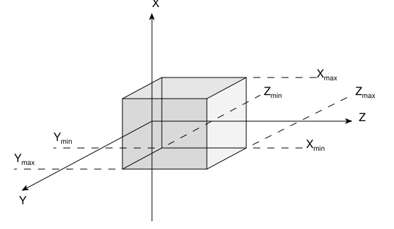
Rectangular Parallelepiped (RPP)
*...+....1....+....2....+....3....+....4....+....5....+....6....+....7..
  RPP    4     -20.0     +20.0     -50.0     +50.0     -38.5     +38.5
* (a parallelepiped centred on the origin)
*...+....1....+....2....+....3....+....4....+....5....+....6....+....7....+.
  RPP    4                 -20.0                 +20.0                 -50.0
                           +50.0                 -38.5                 +38.5
RPP SmlBrick -20.0 +20.0 -50.0 +50.0 -38.5 +38.5
General Rectangular Parallelepiped. Code: BOX
BOX (Fig. 8.2) is also a Rectangular Parallelepiped, but with arbitrary orientation in space. Its use is generally not recommended, since it can be replaced by a suitable combination of infinite planes (PLA, XYP, XZP, YZP). Planes are easier to define, make tracking more accurate and often only a few are needed in a region description.BOX is defined by 12 numbers in the following order: \(V_x\), \(V_y\), \(V_z\) (coordinates of a vertex), \(H^{(1)}_x\), \(H^{(1)}_y\), \(H^{(1)}_z\), \(H^{(2)}_x\), \(H^{(2)}_y\), \(H^{(2)}_z\), \(H^{(3)}_x\), \(H^{(3)}_y\), \(H^{(3)}_z\) (x-, y- and z- components of three mutually perpendicular vectors representing the height, width and length of the box). Note that it is the user’s responsibility to ensure perpendicularity. This is best attained if the user has chosen high-accuracy input fixed format (IDBG = -10 or -100 in the CG Title line, see Geometry Title line), or free format, and the value of each vector component is expressed with the largest available number of significant digits.BOX definition extends over 2 lines in default fixed format, or over 4 lines in high-accuracy body fixed format.*...+....1....+....2....+....3....+....4....+....5....+....6....+....7..
BOX 18 0.0 0.0 0.0 7.0710678 7.0710678 0.0
-14.142136 14.142136 0.0 0.0 0.0 30.0
* (a parallelepiped with a corner on the origin, with edges 10, 20 and
* 30 cm long, rotated counterclockwise by 45 degrees in the x-y plane)
*...+....1....+....2....+....3....+....4....+....5....+....6....+....7....+.
  BOX   18                   0.0                   0.0                   0.0
               7.071067811865475     7.071067811865475                   0.0
              -14.14213562373095     14.14213562373095                   0.0
                             0.0                   0.0                  30.0
*...+....1....+....2....+....3....+....4....+....5....+....6....+....7....+.
BOX tiltslab  0.0  0.0  0.0  7.071067811865475  7.071067811865475  0.0
            -14.14213562373095  14.14213562373095  0.0  0.0  0.0  30.0
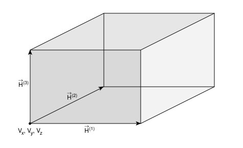
General Rectangular Parallelepiped (BOX)
Sphere. Code: SPH
SPH (Fig. 8.3) is defined by 4 numbers: \(V_x\), \(V_y\), \(V_z\) (coordinates of the centre), \(R\) (radius).SPH definition extends over one single line in default fixed format, or over two lines in high-precision body fixed format.*...+....1....+....2....+....3....+....4....+....5....+....6....+....7..
SPH 002 5.0 -30.0 27.0 528.2
* (a sphere centred at point x=5, y=30, z=27, with a radius of 528.2 cm)
*...+....1....+....2....+....3....+....4....+....5....+....6....+....7....+.
  SPH  002                   5.0                 -30.0                  27.0
                           528.2
SPH TheBall 5.0 -30.0 27.0 528.2
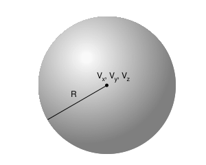
Sphere (SPH)
Right Circular Cylinder. Code: RCC
RCC (Fig. 8.4) can have any orientation in space. It is limited by a cylindrical surface and by two plane faces perpendicular to its axis. (If the cylinder axis is parallel to one of the coordinate axes, it is worth considering instead the use of an infinite cylinder XCC, YCC or ZCC (see below), leading to increased tracking speed).RCC is defined by 7 numbers: \(V_x\), \(V_y\), \(V_z\) (coordinates of the centre of one of the circular plane faces), \(H_x\), \(H_y\), \(H_z\) (x-, y- and z- components of a vector corresponding to the cylinder height, pointing to the other plane face), \(R\) (cylinder radius).RCC definition extends over 2 lines in default fixed format, or over 3 lines in high-accuracy body fixed format.*...+....1....+....2....+....3....+....4....+....5....+....6....+....7..
RCC 07 5.0 5.0 5.0 57.735027 57.735027 57.735027
37.
* (a circular cylinder 100 cm long and of 37 cm radius, with base
* centred at point x=5, y=5, z=5, its axis making equal angles to
* the three coordinate axes).
The same example in high-accuracy body fixed format:
*...+....1....+....2....+....3....+....4....+....5....+....6....+....7....+.
  RCC   07                   5.0                   5.0                   5.0
               57.73502691896258     57.73502691896258     57.73502691896258
                             37.
The same cylinder, in free format:
RCC  BYGCYL  5.0  5.0  5.0  57.73502691896258  57.73502691896258
        57.73502691896258  37.
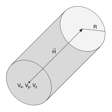
Right Circular Cylinder (RCC)
Right Elliptical Cylinder (REC)
Right Elliptical Cylinder. Code: REC
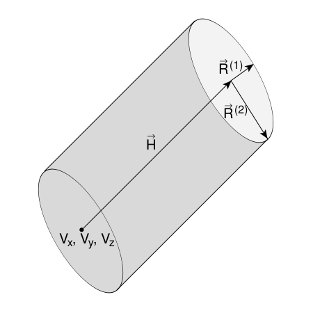
REC (Fig. 8.5) can have any orientation in space. It is limited by a cylindrical elliptical surface and by two plane faces perpendicular to its axis. (If the cylinder axis is parallel to one of the coordinate axes, it is worth considering instead the use of an infinite cylinder XEC, YEC or ZEC (see below), leading to increased tracking speed).REC is defined by 12 numbers: \(V_x\), \(V_y\), \(V_z\) (coordinates of the centre of one of the elliptical plane faces), \(H_x\), \(H_y\), \(H_z\) (x-, y- and z- components of a vector corresponding to cylinder height, pointing to other plane face), \(R^{(1)}_x\), \(R^{(1)}_y\), \(R^{(1)}_z\) (components of a vector corresponding to the minor half-axis of the cylinder elliptical base), \(R^{(2)}_x\), \(R^{(2)}_y\), \(R^{(2)}_z\) (ditto for the major half-axis).REC definition extends over 2 lines in default fixed format, or over 4 lines in high-accuracy body fixed format.*...+....1....+....2....+....3....+....4....+....5....+....6....+....7..
REC 1 -10.0 12.0 7.0 0.0 58.0 0.0
9. 0.0 0.0 0.0 0.0 17.0
* (an elliptical cylinder 58 cm long parallel to the y axis, with minor
* half-axis 9 cm long parallel to the x coordinate axis, major
* half-axis 17 cm long parallel to the z axis, base centred at point
* x=-10, y=12, z=7)
The same example in high-accuracy body fixed format:
*...+....1....+....2....+....3....+....4....+....5....+....6....+....7....+.
  REC    1                 -10.0                  12.0                   7.0
                             0.0                  58.0                   0.0
                              9.                   0.0                   0.0
                             0.0                   0.0                  17.0
The same, in free format:
REC pipesurf -10.0 12.0 7.0 0.0 58.0 0.0 9.0 0.0 0.0 0.0 0.0 17.0
Truncated Right Angle Cone. Code: TRC
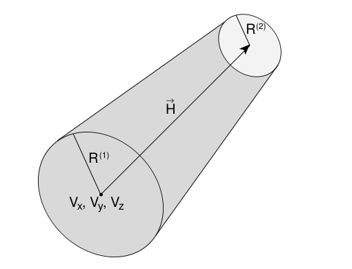
TRC (Fig. 8.6) can have any orientation in space. It is bounded by a conical surface and by two circular plane faces perpendicular to the axis of the cone.TRC is defined by 8 numbers: \(V_x\), \(V_y\), \(V_z\), (coordinates of the centre of the major circular base), \(H_x\), \(H_y\), \(H_z\) (components of a vector corresponding to the TRC height, directed from the major to the minor base), \(R^{(1)}\) (radius of the major base), \(R^{(2)}\) (radius of the minor base)TRC definition extends over 2 lines in default fixed format, or over 3 lines in high-accuracy body fixed format.*...+....1....+....2....+....3....+....4....+....5....+....6....+....7..
TRC 102 0.0 0.0 -130.0 0.0 0.0 1000.0
600. 150.0
* (a truncated cone 1000 cm long parallel to the z axis, with the
* larger circular base 600 cm in radius located at z = -130 and the
* smaller base 150 cm in radius located at z = 870)
The same example in high-accuracy body fixed format:
*...+....1....+....2....+....3....+....4....+....5....+....6....+....7....+.
  TRC  102                   0.0                   0.0                -130.0
                             0.0                   0.0                1000.0
                            600.                 150.0
The same, in free format:
TRC NewCone 0.0 0.0 -130.0 0.0 0.0 1000.0 600. 150.0
Truncated Right Angle Cone (TRC)
Ellipsoid of Revolution. Code: ELL
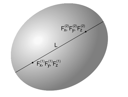
ELL (Fig. 8.7) is a prolate (cigar-shaped) ellipsoid, obtainable by revolution of an ellipse around its major axis, and having any orientation in space.ELL is defined by 7 numbers: \(F^{(1)}_x\), \(F^{(1)}_y\), \(F^{(1)}_z\), \(F^{(2)}_x\), \(F^{(2)}_y\), \(F^{(2)}_z\), (coordinates of the two foci on the major ellipsoid axis), \(L\) (full length of the major axis).ELL definition extends over 2 lines in default fixed format, or over 3 lines in high-accuracy body fixed format.*...+....1....+....2....+....3....+....4....+....5....+....6....+....7..
ELL 003 -400.0 0.0 0.0 400.0 0.0 0.0
1000.
* (an ellipsoid obtained by revolution around the x axis of an ellipse
* centred at the origin, with major axis parallel to x 1000 cm long and
* minor axis 600 cm long).
The same example in high-accuracy body fixed format:
*...+....1....+....2....+....3....+....4....+....5....+....6....+....7....+.
  ELL  003                -400.0                   0.0                   0.0
                           400.0                   0.0                   0.0
                           1000.
ELL TheCigar -400.0 0.0 0.0 400.0 0.0 0.0 1000.0
Ellipsoid of Revolution (ELL)
Right Angle Wedge. Code: WED or RAW
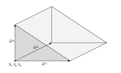
WED (Fig. 8.8) is the half of a BOX (see), cut by a plane passing through its centre and through four corners. Its use, like that of the BOX, is now mostly superseded by the availability of infinite planes and it is therefore deprecated (XYP, XZP, YZP and PLA).WED is defined by 12 numbers: \(V_x\), \(V_y\), \(V_z\) (coordinates of one of rectangular corners), \(H^1_x\), \(H^1_y\), \(H^1_z\), \(H^2_x\), \(H^2_y\), \(H^2_z\), \(H^3_x\), \(H^3_y\), \(H^3_z\) (x-, y- and z- components of three mutually perpendicular vectors corresponding to the height, width and length of the wedge). Note that it is the user’s responsibility to ensure perpendicularity. This is best attained if the user has chosen high-accuracy input format (IDBG = -10 or -100 in the CG Title line, see Geometry Title line), or free format, and the value of each vector component is expressed with the largest available number of significant digits.WED definition extends over 2 lines in default fixed format, or over 4 lines in high-accuracy body fixed format.*...+....1....+....2....+....3....+....4....+....5....+....6....+....7..
WED 97 0.0 0.0 0.0 7.0710678 7.0710678 0.0
-14.142136 14.142136 0.0 0.0 0.0 30.0
* (the bottom half of a parallelepiped with a corner on the origin,
* with edges 10, 20 and 30 cm long, rotated counterclockwise by 45
* degrees in the x-y plane)
*...+....1....+....2....+....3....+....4....+....5....+....6....+....7....+.
  WED   97                   0.0                   0.0                   0.0
               7.071067811865475     7.071067811865475                   0.0
              -14.14213562373095     14.14213562373095                   0.0
                             0.0                   0.0                  30.0
WED  halfbox1  0.0  0.0  0.0  7.071067811865475  7.071067811865475
     0.0  -14.14213562373095  14.14213562373095  0.0  0.0  0.0  30.0
Right Angle Wedge (WED or RAW)
Arbitrary Convex Polyhedron. Code: ARB
ARB (Fig. 8.9) is a portion of space bounded by 4, 5 or 6 plane faces. Its use is rather complicated and is now superseded by the availability of infinite planes (XYP, XZP, YZP and PLA). Please avoid using it as much as possible. For completeness, however, a description of input will be reported here.ARB definition extends over 5 lines in default fixed format, or over 10 lines in high-accuracy body fixed format.*...+....1....+....2....+....3....+....4....+....5....+....6....+....7..
ARB 5 -44.2 -36.5 3572.0 -44.2 -33.5 3572.0
-37.1 -31.0 3572.0 -37.1 -39.0 3572.0
-44.2 -36.5 0.0 -44.2 -33.5 0.0
-37.1 -31.0 0.0 -37.1 -39.0 0.0
1234. 1562. 5876. 1485. 4378. 6732.
* (a right prism of trapezoidal base, of height 3572 cm parallel to the
* z axis)
*...+....1....+....2....+....3....+....4....+....5....+....6....+....7....+.
  ARB    5                 -44.2                 -36.5                3572.0
                           -44.2                 -33.5                3572.0
                           -37.1                 -31.0                3572.0
                           -37.1                 -39.0                3572.0
                           -44.2                 -36.5                   0.0
                           -44.2                 -33.5                   0.0
                           -37.1                 -31.0                   0.0
                           -37.1                 -39.0                   0.0
                            1234.                1562.                 5876.
                            1485.                4378.                 6732.
ARB oddbody -44.2 -36.5 3572.0 -44.2 -33.5 3572.0 -37.1 -31.0 3572.0 -37.1
         -39.0 3572.0 -44.2 -36.5 0.0 -44.2 -33.5 0.0 -37.1 -31.0 0.0 -37.1
         -39.0 0.0 1234. 1562. 5876. 1485. 4378. 6732.
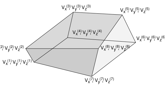
Arbitrary Convex Polyhedron (ARB)
(Truncated) rectangular Pyramid. Code: PYX,PYY,PYZ
PYX (PYY, PYZ) is a pyramid parallel to the x (y, z) axis. It Can be full or truncated.PYX (PYY, PYZ) is defined by 7 numbers: \(V_x\), \(V_y\), \(V_z\), (coordinates of the centre of the major rectangular base), \(L_y\), \(L_z\), (resp. \(L_z\), \(L_x\), or \(L_x\), \(L_y\)) (half-lengths of the sides of the major base), \(H\), (height of the pyramid. The sign gives the direction from major to minor basis), \(R\), (ratio between the sides of the minor base and the sides of the major base. If R=0.0, the pyramid is not truncated. R>=1. is not accepted)PYX (PYY, PYZ) definition extends over 2 lines in default fixed format, or over 3 lines in high-accuracy body fixed format.PYZ body3 0.0 0.5 -10.0 +20.0 +40.0 50.0 0.8
* (a truncated pyramid with major base centered at 0.0, 0.5,-10.0
* and extending from x=-20.0 to x=+20, and from y=-39.5 to y=40.5.
* Its axis is along z, its height is 50 cm, the minor basis extends
* from -16.0 to +16.0 in x and from -31.5 to 32.5 in y)
Infinite half-space delimited by a coordinate plane. Code: XYP, XZP, YZP
There are 4 kinds of infinite half-spaces. Three of them are delimited by planes perpendicular to the coordinate axes:
Delimited by a plane perpendicular to the x-axis. Code:
YZPDelimited by a plane perpendicular to the y-axis. Code:
XZPDelimited by a plane perpendicular to the z-axis. Code:
XYP
YZP, XZP, XYP (Fig. 8.10) definition, in fixed format, extends always over a single line.*...+....1....+....2....+....3....+....4....+....5....+....6....+....7..
YZP 71 -44.2
XZP 72 108.0
XYP 73 0.0
* (respectively, all points having x < -44.2, those having y < 108,
* and those having z < 0)
The same example in high-accuracy body fixed format:
*...+....1....+....2....+....3....+....4....+....5....+....6....+....7....+.
  YZP   71                 -44.2
  XZP   72                 108.0
  XYP   73                   0.0
The same example in free format:
YZP  horizPla  -44.2
XZP  vertPla1   108.0
XYP  vertPla2     0.0
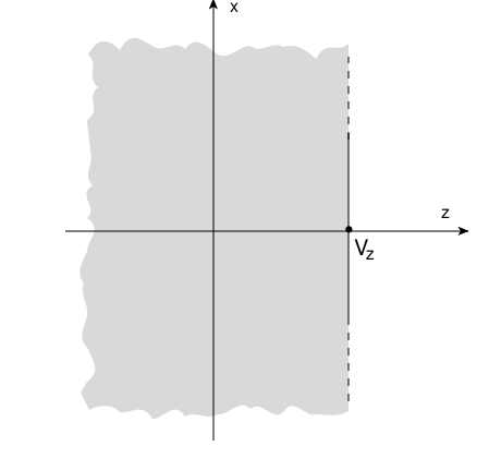
Infinite half-space delimited by a plane perpendicular to the z axis (XYP)
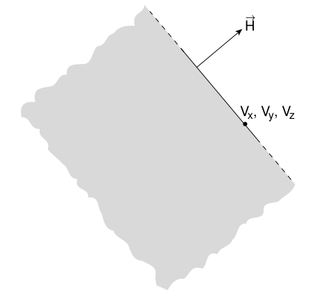
Infinite half-space delimited by a generic plane (PLA)
Generic infinite half-space. Code: PLA
PLA (Fig. 8.11) is defined by 6 numbers: \(H_x\), \(H_y\), \(H_z\) (x-, y- and z- components of a vector of arbitrary length perpendicular to the plane), \(V_x\), \(V_y\), \(V_z\) (coordinates of any point lying on the plane).PLA definition extends over a single line in default fixed format, and over two lines in high-accuracy body fixed format.*...+....1....+....2....+....3....+....4....+....5....+....6....+....7..
PLA 74 0.0 1.0 1.0 200.0 -300.0 240.0
* (all points "below" a plane at 45 degrees in the y-z projection which
* passes through the point x=200, y=-300, z=240 - note that for such a
* plane the x value of the point is completely irrelevant - )
The same example in high-accuracy body fixed format:
*...+....1....+....2....+....3....+....4....+....5....+....6....+....7....+.
  PLA   74                   0.0                   1.0                   1.0
                           200.0                -300.0                 240.0
The same plane in free format:
PLA tiltPla 0.0 1.0 1.0 200.0 -300.0 240.0
Infinite Circular Cylinder parallel to a coordinate axis. Code: XCC, YCC, ZCC
XCC (YCC, ZCC) is an infinite circular cylinder parallel to the x (y, z) axis.XCC (YCC, ZCC) (Fig. 8.12) is defined by 3 numbers: \(A_y\), \(A_z\) (\(A_z\), \(A_x\) for YCC, \(A_x\), \(A_y\) for ZCC) (coordinates of the cylinder axis), \(R\) (cylinder radius)XCC (YCC, ZCC) definition, in fixed format, extends always over one single line.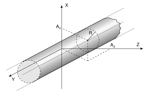
Infinite Circular Cylinder parallel to the y-axis (YCC)
Example in default fixed format:
*...+....1....+....2....+....3....+....4....+....5....+....6....+....7..
  XCC  013    -480.0      25.0     300.0
* (an infinite cylinder of radius 300 cm, with axis defined by y=-480,
*  z=25)
  ZCC  014       0.0       0.0       2.5
* (an infinite cylinder of radius 2.5 cm, with axis equal to the z axis)
The same example in high-accuracy body fixed format:
*...+....1....+....2....+....3....+....4....+....5....+....6....+....7....+.
  XCC  013                -480.0                  25.0                 300.0
  ZCC  014                   0.0                   0.0                   2.5
The same, in free format:
XCC  Column  -480.0  25.0  300.0
ZCC  Tunnel   0.0   0.0    2.5
Infinite Elliptical Cylinder parallel to a coordinate axis. Code: XEC, YEC, ZEC
XEC (YEC, ZEC) is an infinite elliptical cylinder parallel to the x (y, z) axis, and with the axes of the ellipse parallel to the other two coordinate axes.XEC (YEC, ZEC) is defined by 4 numbers: \(A_y\), \(A_z\), (\(A_z\), \(A_x\) for YEC, \(A_x\), \(A_y\) for ZEC) (coordinates of the cylinder axis), \(L_y\), \(L_z\) (\(L_z\), \(L_x\) for YEC, \(L_x\), \(L_y\) for ZEC) (semiaxes of the ellipse).XEC (YEC, ZEC) definition extends over one single line in default fixed format, and over two lines in high-accuracy body fixed format.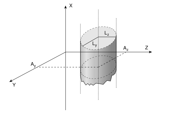
Infinite Elliptical Cylinder parallel to the x-axis (XEC)
Example in default fixed format:
*...+....1....+....2....+....3....+....4....+....5....+....6....+....7..
  ZEC  101      15.0     319.0      33.0      80.0
* (an infinite elliptical cylinder, centred on x=15, y=319, with the
* ellipse minor semi-axis parallel to x, 33 cm long, and the major
* semi-axis parallel to y, 80 cm long)
The same example in high-accuracy body fixed format:
*...+....1....+....2....+....3....+....4....+....5....+....6....+....7....+.
  ZEC  101                  15.0                 319.0                  33.0
                            80.0
The same body, described in free format:
ZEC ChimneyA 15.0 319.0 33.0 80.0
Generic Quadric. Code: QUA
QUA is a quadric surface defined by a \(2^{nd}\) degree equation \(F(x,y,z) = 0.\)QUA is defined by 10 numbers:QUA definition extends over two lines in default fixed format, and over 4 lines in high-accuracy body fixed format.*...+....1....+....2....+....3....+....4....+....5....+....6....+....7..
QUA 27 0.0025 0.04 0.0064 0.0 0.0 0.0
0.055 0.64 0.0256 1.8881
* (an ellipsoid centred at x = -11 cm, y = -8 cm, z = -2 cm, with
* a semi-axis 20 cm long parallel to x, one 5 cm long parallel to y and
* one 12.5 cm long parallel to z)
The same example in high-accuracy body fixed format:
*...+....1....+....2....+....3....+....4....+....5....+....6....+....7....+.
  QUA   27                0.0025                  0.04                0.0064
                             0.0                   0.0                   0.0
                           0.055                  0.64                0.0256
                          1.8881
The same body, described in free format:
QUA Elipsoid 0.0025 0.04 0.0064 0.0 0.0 0.0 0.055 0.64 0.0256 1.8881
NOTE
Generic tetrahedron. Code: TET
A TET has four faces and four vertices and is defined by twelve parameters: the three coordinates of each vertex \(V_a\), \(V_b\), \(V_c\), \(V_d\). The vertices of each face must appear counterclockwise when viewed from outside the tetrahedron, in these orders:
first face: \(V_a,V_b,V_c\);
second face: \(V_a,V_c,V_d\);
third face: \(V_a,V_d,V_b\);
fourth face: \(V_b,V_d,V_c\).
Plotting the tetrahedron on paper makes this numbering easier to visualise. Example:
TET BdTetr    0.0  0.0  1.0
             0.0  0.0  0.0
             1.0  0.0  0.0
             0.0  1.0  0.0
Summary
These should indeed make tracking faster, since for them extra coding ensures that unnecessary boundary intersection calculations are avoided when the length of the next step is smaller than the distance to any boundary of the current region.
Geometry directives
$Start_xxx ....... $End_xxxxxx stands for expansion, translat or transform. They allow to provide respectively a coordinate expansion, a coordinate translation and a coordinate roto-translation of the bodies embedded between the starting and the ending directive lines. Directives can be nested.The body definitions which are contained between the lines $Start_xxx and $End_xxx are automatically modified according to the syntax described below.
Expansion
This directive provides a coordinate expansion (or reduction) of the body dimensions by a defined scaling factor, for all bodies embedded between the two lines.
$Start_expansion [scaling factor]
..............
..............
..............
$End_expansion
Example:
$Start_expansion 10.
QUA  Elipsoid  0.0025 0.04 0.0064 0.0 0.0 0.0 0.055 0.64 0.0256 1.8881
$End_expansion
transforms an ellipsoid centred at (-11, -8, -2), with semiaxes 20, 5 and 12.5 cm long parallel to the coordinate axes, to one centred at (110, 80, -20) with semiaxes 200, 50 and 125 cm long.
Translation
This directive provides a coordinate translation. The bodies embedded between th e two lines are translated by [dX] [dY] [dZ] on the three axes.
$Start_translat [dX] [dY] [dZ]
..............
..............
..............
$End_translat
Example:
$Start_translat -5., -7., +9.
QUA  Elipsoid  0.0025 0.04 0.0064 0.0 0.0 0.0 0.055 0.64 0.0256 1.8881
$End_translat
transforms an ellipsoid centred at (-11, -8, -2), with semiaxes 20, 5 and 12.5 cm long parallel to the coordinate axes, to an identical one centred at (6, 1, 7)
Roto-translation transformation
This directive provides a coordinate transformation, predefined by a ROT–DEFIni card, for all bodies embedded between the two lines.
$Start_transform [ROT-DEFIni name] (or [ROT-DEFIni number])
..............
..............
..............
$End_transform
Two nested (signed) transformations R2 and R1 can be used, acting on a body vector \(\mathbf{r}\) as \(\mathbf{r}'=R_2R_1\mathbf{r}\):
$Start_transform R2
...
$Start_transform R1
...
$End_transform
...
$End_transform
Example 1:
....
* Cylindrical target is transformed with  transformation "Rotdefi1"
$Start_transform  Rotdefi1
RCC targRepl   0.0 0.0 -5.0 0.0 0.0 10.0 5.0
$End_transform
....
* ROT-DEFI transformations shift of (0,-2,-30) then rotation of -21 degrees
* around the x axis
ROT-DEFI         0.0                                    -2.0     -30.0Rotdefi1
ROT-DEFI        100.                -21.                              Rotdefi1
Example 2 (with lattice):
....
* Cylindrical target
RCC target     0.0 0.0 -5.0 0.0 0.0 10.0 5.0
* Target replica is transformed with inverse transformation of the lattice
$Start_transform  -Rotdefi1
RCC targRepl   0.0 0.0 -5.0 0.0 0.0 10.0 5.0
$End_transform
....
* Regions
TARGET       5 +target
REPLICA      5 +targRepl
....
* Lattice
LATTICE      REPLICA                                                  Rotdefi1
....
* ROT-DEFI transformation: shift of (0,-2,-30) then rotation of -21 degrees
* around the x axis
ROT-DEFI         0.0                                    -2.0     -30.0Rotdefi1
ROT-DEFI        100.                -21.                              Rotdefi1
Example 3:
ROT-DEFIni  3. -90.  0.  0.  0.  0. XtoZ
........................................
$Start_transform XtoZ
$Start_translat 0. -30. +20.
$Start_expansion 10.
QUA  Elipsoid  0.0025 0.04 0.0064 0.0 0.0 0.0 0.055 0.64 0.0256 1.8881
$End_expansion
$End_translat
$End_transform
transforms an ellipsoid centred at (-11, -8, -2), with semiaxes 20, 5 and
12.5 cm long parallel to the coordinate axes, to a similar one with
semiaxes 200, 50 and 125 cm, centred at (11, -22, 18) and rotated by 90
degrees (axis z becomes axis x).  Note that $Start_expansion takes
precedence over $Start_translat, which in turn takes precedence over
$Start_transform.
Example 4: Trivial example where the combined nested transformation is the identity. The first transformation (ft) is a rotation by 90 deg around the y axis, followed by a shift of 10 cm along the z axis. The second transformation is the inverse: a shift of -10 cm along the z axis and a rotation of -90 deg around the y axis.
ROT-DEFI        200.                 90.                              ft
ROT-DEFI         0.0                                               10.ft
ROT-DEFI         0.0                                              -10.st
ROT-DEFI        200.                -90.                              st
$start_transform st
$start_transform ft
* Cylindrical target
RCC target     0.0 0.0 0.0 0.0 0.0 10. 2.
$end_transform
$end_transform
Geometry directives: usage notes
$Start_expansion takes precedence over $Start_translat, which in turn takes precedence over $Start_transform.
Directives $Start_expansion and $Start_translat are applied when reading the geometry: therefore they imply no CPU penalty. Directive $Start_transform, instead, is applied at run-time and requires some additional CPU time.
Directives can be nested. All the directives can be used in association with lattices.
The ROT–DEFIni cards are used by the geometry directive to transform the coordinates of the bodies (not of the particles!). If a “-” sign is placed in front of the [ROT-DEFIni name or number] of the $Start_transform directive the inverse transformation is used instead.
Body END line
Body definitions must be terminated by a line with the string END (in column 3–5 if fixed format is used).
.98
Region data
The various regions are described in terms of differences, intersections and unions of bodies. As in the case of body description, the user has the choice between free format and two kinds of fixed format. One of the latter is the traditional format used by the original Combinatorial Geometry as implemented for example in MORSE. The other fixed format is similar to it, but has been extended to allow body numbers larger than 10000. Both fixed formats are now superseded by the more convenient free region input format, recently introduced. Free format is based on body mnemonic “names” instead of sequential numerical identifiers and allows the use of parentheses to perform more complex boolean operations. However, the two fixed formats are still available for back compatibility reasons.
With any input format, a line having an asterisk (*) in column 1 is treated as a comment card.
Fixed format region input
Each region is described as a combination of one or more bodies, by means of the three operator symbols:
and OR
referring respectively to the boolean operations of subtraction (or complement), intersection and union.
IDBG on the Geometry Title line (see Geometry Title line).IDBG = 0, 10 or -10, region input format is (2X,A3,I5,9(A2,I5));IDBG = 100 or -100, region input format is (2X,A3,I5,7(A2,I7));on the first input line of a given region, an arbitrary non-blank string chosen by the user (it can be used, together with optional comment lines, to help identifying the region or the region material).
Note that regions are identified in the code by an integer number corresponding to the order of their input definition: therefore it can be useful (but not mandatory) to have that number appearing in the string. For instance, if the 5th region is air, it could be labelled AI5.
on all continuation lines, columns 3-5 must be blank.
NAZ):is the number of regions which can be entered by a particle leaving any of the bodies defined for the region being described (leave blank in continuation lines). The
NAZ number is used to allocate memory for this so-called “contiguity list”, and it is not essential that it be exact (if left blank, it is set to 5). Any number is accepted, but if the final sum of these integers is close to the actual sum, tracking speed can be slightly improved.
alternate as many 2-character fields (’
OR’ or blank) and integer fields (body numbers preceded by+or-sign), as are needed to complete the description of that region (see below for an explanation of symbol meaning). If one line is not sufficient, any number of continuation lines can be added (identified by a blank field in column 3–5).
After the last region description, end with a line having the code END in columns 3–5.
Meaning of the + - OR operators
+ operator, it means that the zone being described is wholly contained inside the body.- operator, it means that the zone being described is wholly outside the body.+ must appear at least once.*...+....1....+....2....+....3....+....4....+....5....+....6....+....7..
BA1 4 +7 +3
* (the above region is the part of space common to body 7 and 3)
MU2 7 +3 -4 -7 +20
* (the above region is the part of space common to body 3 and 20,
* excluding however that which is inside body 4 and that which is
* inside 7)
AIR 5 +19
* (the latter region coincides entirely with body 19)
OR operator is used as a boolean union operator in order to combine subregions (partially overlapping or not). Subregions (also called “zones” in this manual) are formed as intersections or differences as explained above, and then the region is formed by a union of these subregions. When OR operators are used there are always two or more of them, and they refer to all body numbers following them until the next OR or the end of the region description, each body being preceded by its + or - sign.*...+....1....+....2....+....3....+....4....+....5....+....6....+....7...
SA7 11OR +4 +6 -7 -8OR +6 +3 -21
* <---- first subregion -----><- second subregion ->
G18 2OR +9OR +15OR +1OR +8 -2OR +8 -3OR +8 +18
* < 1st >< 2nd >< 3rd ><--- 4th ----><--- 5th ----><--- 6th ---->
OR +12 -10 -11 -13 -14
*< blank ><---- 7th and last subregion -----> (continuation line)
Free format region input
Each region is described as a combination of one or more bodies, by means of the three operator symbols:
and |
REGNAME, NAZ and the remaining part are separated by one or more blanks.REGNAMEis the region “name” (an arbitrary unique alphanumeric character string chosen by the user). The region name must begin by an alphabetical character and must not be longer than 8 characters.NAZ is an integer indicating (approximately) the number of regions which can be entered by a particle leaving any of the bodies appearing in the region description that follows. TheNAZnumber is used to allocate memory for this so-called “contiguity list”, and it is not essential that it be exact. Any number is accepted, but if the final sum of these integers is close to the actual sum, tracking speed can be slightly improved. In free format input,NAZmay not be left blank.If
NAZis negative is enforcing the use ofDNEAR(see GLOBAL card) for that specific zone, which will result in more efficient tracking in this zone.If
NAZis positive the use ofDNEARwill be decided by the code depending or not the existance of overlapping zones.
- “boolean-zone-expression” is a sequence of one or more body names preceded by the operators
+(intersection) or-(complement or subtraction). A zone expression can be contained inside one or more sets of left and right parentheses. Several zone expressions can be combined by the union operator|(corresponding toORin fixed format input).When|operators are used there are always two or more of them, and they refer to all bodies following them until the next|or the end of the region description, each body being preceded by its+or-sign.In evaluating the expressions, the highest operator precedence is given to parentheses (the most inner ones first), followed by the|operator. In each zone expression, at least one body name preceded by+must be present. If one line is not sufficient, any number of continuation lines can be added. Blanks are ignored.
Region description ends with a line containing the single string END.
Meaning of the + - | operators
If a body name is preceded by a
+operator in an expression describing a zone (or a zone component surrounded by parentheses) it means that the zone or zone component being described is wholly contained inside the body (boolean intersection).If a body name is preceded by a
-operator in an expression describing a zone (or a zone component surrounded by parentheses) it means that the zone or zone component being described is wholly outside the body (boolean complement).
Obviously, in the description of each region the symbol + must appear at least once. The same is true for each zone (subregion delimited by | operators) and for each zone component (subzone delimited by parentheses)
lastlayr   4  +bigball  +slab
* Region "lastlayr" is the part of space common to body "bigball" and body
* "slab"

MidVacuu  7 +cylind2   -slit  -sqrhole +Plane1
* Region "MidVacuu" is the part of space common to bodies "cylind2" and
* "Plane1", excluding however that which is inside body "slit" and that which
* is inside body "sqrhole"

H2Osphere   5   +marble
* Region "H2Osphere" coincides entirely with body "marble"
Examples of regions consisting of the union of several zones, possibly (but not necessarily) partially overlapping:
Corners  6 | +dice +topNorth | +dice +topEast | +dice +topSouth |
+dice +topWest | +dice +botNorth | +dice +botEast | +dice +botSouth | +dice
+botWest
* Region "Corners" is made of the 8 corners of a cube, each of which is
* obtained by the intersection of a cubic body "dice" and a tilted plane
* described by vector pointing to the centre of the cube

twoparts 0 | +leftpart -outerbox | +rghtpart +topplane
* Region "twoparts" is the sum of two parts of space: the space points which
* are inside body "leftpart" but not inside body "outerbox", plus those which
* are common to bodies "rghtpart" and "topplane"
Examples of a region defined as a single zone by means of parentheses:
AirAroun 5  + tunnel + Column - (+outrpipe-innrpipe)
* Region "AirAroun" contains the space points located inside the intersection
* of body "tunnel" and body "Column", with the exception of those which are
* inside body "outrpipe" but not inside body "innrpipe"

CmplexRg | +longcyl + (+shortcyl +vertPla1 -vertPla2) | (+Brick | + ceeling
- floor)
* Region CmplexRg is the union of two zones. The first zone is the
* intersection of body "longcyl" with a portion of space contained inside
* both bodies "shortcyl" and "vertPla1" but not inside body "vertPla2".
* The second zone is the union of the space points inside body "Brick"
* and the space points contained by body  "ceeling" but located outside
* body "floor".
Region END line
Region data must be terminated by a line with the string END (in column 3–5 if format is fixed).
Region Volumes
This is an optional set of cards which must be input if (and only if) flag IVLFLG in the CG Title line has been given a value 3 (see Geometry Title line). As many volume definition cards must be given as is needed to input a volume for every region. The input variable is an array VNOR(I) = volume of the Ith region. The format is (7E10.5). Volume data are used by FLUKA only to normalise energy or star densities per region, requested by the SCORE command.
LATTICE card
This is an optional card for modular geometries. Its use needs some more effort and preparation.
The basic unit of the geometry, composed by an arbitrary number of regions, must be described in full detail in the body and region data.
Additional body and region data must also be provided to describe “container” regions representing the “boxes”, or lattice cells, wherein the basic unit has to be replicated. No material assignment is needed for these lattice-cell regions.
A roto-translation must be defined (option
ROT–DEFIand associated with each lattice to provide the transformation bringing from any point and direction inside each lattice cell to the corresponding point and direction in the basic unit. Alternatively, a user routine (LATTIC, see LATTIC: (symmetry transformation for lattice geometry)) can be written for the same purpose.The
LATTICEcard itself identifies the lattice cells and establishes the correspondence between region number and lattice cell number, where the region number is the sequential number in the region table, and the lattice cell number is that used in the tracking to address the transformation routine, and is chosen by the user. Contiguous numbering is recommended for memory management reasons, but is not mandatory. Non-contiguous numbering can be done using severalLATTICEcards.
In the LATTICE card, the meanings of the WHAT parameters are:
- WHAT(1) =
- “Container-region” number of the first lattice cell(“From region ``WHAT(1)``…”)
- Default
: No default
- WHAT(2) =
- “Container-region” number of the last lattice cell(“…to region ``WHAT(2)``…”)
- Default
=
WHAT(1)- WHAT(3) =
- step length in assigning “Container-region” numbers(“…in steps of ``WHAT(3)`` ”)
- Default
= 1.0
- WHAT(4) =
lattice number of the first lattice cell (or corresponding name), assigned to region
WHAT(1)- Default
: No default
- WHAT(5) =
lattice number of the last lattice cell (or corresponding name), assigned to region
WHAT(2)- Default
: No default
- WHAT(6) =
- step length in assigning cell numbers/names(“…in steps of ``WHAT(6)`` ”)
- Default
= 1.0
- SDUM
= possible index of transformation associated with this lattice. Exceptionally, here
SDUMcan contain an integer number, in free format, following any of the strings “ROT#”, “Rot#”, “rot#”, “RO#”, “Ro#”, “ro#”. If any one of such strings is present, an integer identifying the associated roto-translation is read in the following characters. If no such string is found, theLATTICuser routine will be called whenever a transformation is required. Otherwise, if a name is present, it is supposed to be the (character) name (with sign) of the associated roto-translation. If a null string is found, the LATTIC user routine will be called whenever a transformation is required. It is possible to associate a nested transformation to a lattice (see card LATTSNGL LATTSNGL card).
LATTICE cards may be issued in the same geometry, when different symmetries are present in different areas. In principle, any analytical symmetry transformation can be implemented (rotation, translation, reflection, or combination of these).NOTE: The lattice cell regions do not need to be included in the other input option cards. Materials, thresholds, etc., must be assigned only to the regions contained in the basic unit. Of course, this implies that all copies of a same basic unit share the same material, setting and biasing properties.
IMPORTANT: If the geometry is being described in free format, using alphanumeric names as body and region identifiers, names must be used also in the LATTICE card(s) for both regions and lattices.
LATTSNGL card
This card allows to associate two nested (signed) transformations \(R_1\) and \(R_2\) to a lattice. The resulting nested transformation acts on a body vector \(\mathbf{r}\) as
- WHAT(1) =
“Container-region” number of the lattice cell.
- Default
= No default
- WHAT(2) =
Index or name (with sign) of the first transformation, \(R_1\).
- Default
= 0
- WHAT(3) =
Index or name (with sign) of the second transformation, \(R_2\).
- Default
= 0
- WHAT(4) =
Lattice number of the lattice cell (or corresponding name), assigned to region WHAT(1).
- Default
= No default
- WHAT(5) =
Not used.
- WHAT(6) =
Not used.
- SDUM =
Not used.
GEOEND card
A card with the string GEOEND in column 1–6 must terminate the combinatorial geometry input.
Geometry debugger
GEOEND card can be used also to activate the geometry debugger, using the WHAT and SDUM parameters. In this case, a second GEOEND card (continuation) may be necessary. It is recommended that a STOP card should follow immediately, avoiding to start transport when debugging is completed.GEOEND card:- WHAT(1) =
X\(_{max}\) of the geometry region to be debugged (no default)
- WHAT(2) =
Y\(_{max}\) of the geometry region to be debugged (no default)
- WHAT(3) =
Z\(_{max}\) of the geometry region to be debugged (no default)
- WHAT(4) =
X\(_{min}\) of the geometry region to be debugged (no default)
- WHAT(5) =
Y\(_{min}\) of the geometry region to be debugged (no default)
- WHAT(6) =
Z\(_{min}\) of the geometry region to be debugged (no default)
- SDUM
=
DEBUGto activate the debugger, otherwise must be left blank
Second (optional) GEOEND card:
- WHAT(1) =
Number of mesh intervals in the X-direction between X\(_{min}\) and X\(_{max}\)
- Default
= 20.0
- WHAT(2) =
Number of mesh intervals in the Y-direction between Y\(_{min}\) and Y\(_{max}\)
- Default
= 20.0
- WHAT(3) =
Number of mesh intervals in the Z-direction between Z\(_{min}\) and Z\(_{max}\)
- Default
= 20.0
- WHAT(4) =
Maximum number of errors after which geometry debugging stops.
- Default
= 500.0
- WHAT(5)
– WHAT(6): not used
- SDUM
= “
&” in any position in column 71 to 78 (or in the last field if free format is used)- Default
(option
GEOENDnot given): not allowed!GEOBEGINandGEOENDmust always be present.
See the Notes to GEOEND option (GEOEND) for more details and instructions.
Voxel geometry
It is possible to describe a complex geometry in terms of “voxels” (tiny identical parallelepipeds forming a 3-dimensional grid). In principle this can be done with any geometry but it is especially useful when translating a CT scan of a human body into a dosimetry phantom [Zan01]. Therefore, we will use loosely the word “organ” to indicate a contiguous group of voxels (or even more than one group) made of the same material. The code handles each organ as a Combinatorial Geometry region, possibly in addition to other conventional “non-voxel” regions defined by the user, and assigns automatically to each organ a new region number.
To describe a voxel geometry, the user must:
Assign an organ to each voxel. Each organ is identified by a unique integer ≤ 32767. The numbering does not need to be contiguous, i.e. gaps in the numbering sequence are allowed. One of the organs must have number 0 and plays the role of the medium surrounding the voxels (usually vacuum or air).
The assignment is done via a special file where the organ corresponding to each voxel is listed sequentially in Fortran list-oriented format, with the
xcoordinate running faster thany, andyrunning faster thanz. In practice the file is always written by a program similar to the one reported below. The user will need to modify the values of the parametersDX, DY, DZ, NX, NY, NZ(respectively voxel size and number of voxels for each coordinate), and possibly some other more trivial things (file names, title, reading from the original CT scan file).The following program takes also care of recompacting the original organ numbers by eliminating all gaps in the sequence, and writes a translation table to the screen:
WRITE(*,'(A,2I10)')' New number, old number: ', NO, IC
After having modified the program (assumed to be in a filewritegolem.f), compile it:$FLUPRO/flutil/fff writegolem.flink it with the FLUKA library:$FLUPRO/flutil/lfluka -o writegolem writegolem.oexecute it:./writegolemThe result will be a filegolem.vxl(or equivalent name chosen by the user) which will be referred to by a special command line in the geometry input (see 2 below).PROGRAM WRITEGOLEM INCLUDE '(DBLPRC)' INCLUDE '(DIMPAR)' INCLUDE '(IOUNIT)' * COLUMNS: FROM LEFT TO RIGHT * ROWS: FROM BACK TO FRONT * SLICES: FROM TOP TO BOTTOM PARAMETER ( DX = 0.208D+00 ) PARAMETER ( DY = 0.208D+00 ) PARAMETER ( DZ =-0.8D+00 ) PARAMETER ( NX = 256 ) PARAMETER ( NY = 256 ) PARAMETER ( NZ = 220 ) DIMENSION GOLEM(NX,NY,NZ) INTEGER*2 GOLEM CHARACTER TITLE*80 DIMENSION IREG(1000), KREG(1000) INTEGER*2 IREG, KREG * CALL CMSPPR DO IC = 1, 1000 KREG(IC) = 0 END DO OPEN(UNIT=30,FILE='ascii_segm_golem',STATUS='OLD') READ(30,*) GOLEM NO=0 MO=0 DO IZ=1,NZ DO IY=1,NY DO IX=1,NX IF (GOLEM(IX,IY,IZ) .GT. 0) THEN IC = GOLEM(IX,IY,IZ) MO = MAX (MO,IC) DO IR=1,NO IF (IREG(IR) .EQ. IC) GO TO 1000 END DO NO=NO+1 IREG(NO)=IC KREG(IC)=NO WRITE(*,'(A,2I10)')' New number, old number: ', NO, IC 1000 CONTINUE END IF END DO END DO END DO * NO = number of different organs * MO = max. organ number before compacting WRITE(*,*) ' NO,MO',NO,MO OPEN(UNIT=31,FILE='golem.vxl',STATUS='UNKNOWN',FORM='UNFORMATTED') TITLE = 'Golem' WRITE(31) TITLE WRITE(31) NX,NY,NZ,NO,MO WRITE(31) DX,DY,DZ WRITE(31) GOLEM WRITE(31) (KREG(IC),IC=1,MO) STOP END
Starting from Fluka2011.2b, the voxel files can contain an arbitrary number of extra records of 80 characters each, which are read and interpreted as ordinary input cards. This allows to embed in the voxel files informations such as material definitions, material assignments, correction factor etc, which are often generated by automatic programs out of a CT scan. Flair contains tools for reading CT scans in Dicom format, and automatically generate a voxel file containing the material and correction factor informations according to a Hounsfield number to material/density translation algorithm which can be tuned by the user.
Prepare the usual FLUKA input file. The geometry must be written like a normal Combinatorial Geometry input (in any of the allowed formats, as part of the normal input stream or in a separate file), but in addition must include:
A
VOXELScard as a first line, before the Geometry title card (Geometry Title line), with the following information:WHAT(1), WHAT(2), WHAT(3)=x, y, zcoordinates chosen as the origin of the “voxel volume”, i.e. of a region made of a singleRPPbody (Rectangular Parallelepiped. Code: RPP) which contains all the voxelsWHAT(4)= index (or name) of theROT–DEFInicard for an eventual roto/translation of the VOXELsWHAT(5): not usedWHAT(6): used mainly for debugging. If WHAT(6) is not divisible by 10, a voxel geometry test is carried out. The RPP-to-voxel, voxel-to-organ, and organ-to-region correspondences are checked. The program stops in case of inconsistency.SDUM= name of the voxel file (extension will be assumed to be.vxl)The usual list of
NBbodies, not including theRPPcorresponding to the “voxel volume” (seeVOXELScard above). ThisRPPwill be generated and added automatically by the code as the(NB+1)th body, with one corner in the point indicated in theVOXELScard, and dimensionsNX*DX, NY*DYandNZ*DZas read from the voxel file.The usual region list of
NRregions, with the space occupied by bodyNB+1(the “voxel volume”) subtracted. In other words, theNRregions listed must cover the whole available space, except the space corresponding to the “voxel volume”. This is easily obtained by subtracting bodyNB+1in the relevant region definitions, even though this body is not explicitly input at the end of the body list. The code will automatically generate and add several regions:Name
Number
Description
VOXELNR+1this is a sort of “cage” for all the voxels. Nothing
(energy etc.) should ever be deposited in it: the user
shall assign
VACUUMto itVOXEL001NR+2containing all voxels belonging to organ number 0.
There must be at least 2 of such voxels, but in general
they should be many more. Typical material assignment
to region
NR+2isAIR.VOXEL002NR+3corresponding to organ 1
VOXEL003NR+4corresponding to organ 2
.......................................VOX*****NR+2+NOcorresponding to organ
NOwhere
NO= number of non-zero organs.
The assignment of materials shall be made by command ASSIGNMAt (and in a similar way other region-dependent options) referring to the first NR regions in the usual way, and to the additional regions using the correspondence to organs as explained above.
The Flair Geometry Editor
The Geometry Editor is an addition to Flair (see Flair) for viewing/debugging and editing FLUKA geometries in a graphical way. It works on 2D cross sections of the geometry with some 3D capabilities.
Main features:
Fast display of complex geometries
- Many user-customizable layers:the Layers dialog allows the user to create customized views. The user has the possibility to change the fill color of the regions displaying regions, materials or even color encoding of biasing, cuts, thresholds etc. Moreover the user has the possibility to overlay a background image, e.g. a technical drawing,
USRBINdata,BEAMparameters, lattices, voxels, transformations, as well as 3D representations using a raytracing technique.Or a combination of any of the above. Graphical editing of the bodies with snapping mechanism to generate accurate coordinates
Visual selection and editing of zones without the need to know the orientation of bodies
Use real curve of bodies with no conversion to vertices/edges
Interactive debugging with information of problematic bodies, regions and/or zones