Special source: cosmic rays¶

Cosmic ray calculations can be done with FLUKA using the input commands GCR–SPE (for initialisation purposes) and SPECSOUR. In addition, several auxiliary stand-alone programs need to be used to prepare the geometry and material cards to be inserted into the input file.

Command SPECSOUR does not define only cosmic ray sources, but also a number of other pre-defined complex sources that cannot be described by the simple keywords BEAM, BEAMPOSit, BEAMAXES and HI–PROPErt. To avoid confusion, SPECSOUR input related to cosmic rays is described separately in this Chapter, in The various SDUM options available with command SPECSOUR.

A complete calculation to determine particle fluxes in the atmosphere requires:

the determination of the spectrum and composition of cosmic rays at the local interstellar medium,
the determination of changing conditions in the solar wind magnetic field and the resulting interaction with the inward flow of galactic cosmic rays from the local interstellar medium,
the determination of the trajectories of cosmic rays through the Earth’s geomagnetic field,
the transport of the surviving incident cosmic rays through the Earth’s atmosphere to various depths.

The following options are available concerning the simulation of cosmic ray interactions in FLUKA:

Superposition model. In this approach primary nuclei are split into equivalent independent nucleons. See card PHYSICS with SDUM = IONSPLITti.
DPMJET interaction model [Ran95, Roe01]. This model simulates the nucleus-nucleus collision above 5 GeV/nucleon. In case DPMJET is chosen for cosmic ray application, it is suggested to avoid the otherwise recommended Dpmjet-III choice and to use instead the Dpmjet-II.5 version (linking with the script $FLUPRO/flutil/ldpm2qmd).

The DPMJET and the superposition model can also be used together, by setting the respective energy ranges with the PHYSICS card.

A number of tools and packages have been developed for the FLUKA environment to simulate the production of secondary particles by primary cosmic rays interacting with the Earth’s atmosphere. These tools, in different stand-alone versions, have already been successfully used for fundamental physics research [Bat00, Bat03a].

The set of FLUKA tools for cosmic ray simulation includes a set of core routines to manage event generation, geomagnetic effects and particle scoring, and the following stand-alone data files and programs :

file atmomat.cards: it contains the material definitions for the density profile of the U.S. Standard Atmosphere. These cards must be inserted (or the file included with the #include directive) into the FLUKA input file.
file atmogeo.cards: it contains an example of a 3D geometrical description of the Earth atmosphere, generated in according with the previous data cards (and corresponding density profile). This geometry includes the whole Earth.
program atmloc_2011.f: it prepares the description of the local atmosphere geometry with the atmospheric shells initialised by option GCR–SPE. This geometry includes only a slice of the Earth geometry, centered around the geomagnetic latitude input by the user
files <iz>phi<MV>.spc: GCR All-Particle-Spectra for the $iz_{th}$ ion species (iz = 1, …, 28), modulated for the solar activity corresponding to a $\phi$ parameter <MV> MegaVolt. $\phi = 500$ MV roughly corresponds to solar minimum, while $\phi = 1400$ MV roughly corresponds to solar maximum.
file allnucok.dat: GCR All-Nucleon Spectra
file sep20jan2005.spc: spectra for the Solar Particle Event of Jan 20th, 2005
file sep28oct2003.spc: spectra for the Solar Particle Event of Oct 28th, 2008

Primary spectrum¶

The Galactic Cosmic Ray (GCR) component of the cosmic ray flux can be simulated up to 30 TeV/nucleon (or 500 TeV/n when DPMJET is linked). Three options are available: with the first two the actual ion composition of the flux is used (AMS All-Particle Spectrum, Old All-Particle Spectrum), while with the second option the primary flux is treated as a sum of nucleons (All-Nucleon Spectrum).

The AMS All-Particle Spectrum¶

The ion composition of the Local Interstellar Medium (LIS) is derived from the most recent AMS02 data as described in [DTL22] for all elemental groups from Z = 1 to Z = 28. In some cases, indvidual isotopes for the same Z are explicitly treated as such. A code [Bad96] is then used to apply the solar modulation to the LIS spectra. The spectrum components are written into 33 files. The name of the files has the form (Z+phi+<PhiMV>+.spc). The first two characters of each file name are the atomic number of a different primary spectrum ion (e.g. 01:protons, 02:alpha…). The following two characters determine its mass number, zero means natural isotopic composition. They are followed by the solar modulation parameter used for generating the spectrum (7 characters) and by an extension .spc. The .spc files are spectra without geomagnetic cutoff. The .spc files are used together with various analytical approximations of the rigidity cutoff, according to an offset or centered dipole approximation of the Earth geomagnetic field, adapted to result in the vertical cutoff inserted into the input file (SPECSOUR command, SDUM = GCR–AMS, WHAT(2) of the continuation card), at the geomagnetic latitude and longitude of interest.

The GSF All-Particle Spectrum¶

The ion composition of the Local Interstellar Medium (LIS) is derived from the most recent Global Spline Fit (GSF) as described in [Hpd17] for all elemental groups from Z = 1 to Z = 28. In some cases, indvidual isotopes for the same Z are explicitly treated as such. A code [Bad96] is then used to apply the solar modulation to the LIS spectra as for the HCR-AMS option. The spectrum components are written into 33 files. The name of the files has the form (Z+A+gsf+<PhiMV>+.spc). The first two characters of each file name are the atomic number of a different primary spectrum ion (e.g. 01:protons, 02:alpha…). The following two characters determine its mass number, zero means natural isotopic composition. They are followed by the solar modulation parameter used for generating the spectrum (7 characters) and by an extension “.spc”. The “.spc” files are spectra without geomagnetic cutoff. The “.spc” files are used together with various analytical approximations of the rigidity cutoff, according to an offset or centered dipole approximation of the Earth geomagnetic field, adapted to result in the vertical cutoff inserted into the input file (SPECSOUR command, SDUM=GCR-GSF, WHAT(2) of the continuation card), at the geomagnetic latitude and longitude of interest.

The OLD All-Particle Spectrum¶

The ion composition of the galactic flux is derived from a code [Bad96] which considers all elemental groups from Z = 1 to Z = 28. The spectrum is modified to follow recent data sets (AMS [Alc00, Alc00a] and BESS [San00] data of 1998) up to 100 GeV according to the so-called ICRC2001 fit [Gai01]. The spectrum components are written into 28 files. The name of the files has the form (Z+phi+<PhiMV>+.spc). The first two characters of each file name are the atomic number of a different primary spectrum ion (e.g. 01: protons, 02: alpha…). They are followed by the solar modulation parameter used for generating the spectrum (7 characters) and by an extension .spc.

The .spc files are spectra without geomagnetic cutoff. The .spc files are used together with an analytical calculation of the rigidity cutoff, according to a centered dipole approximation of the Earth geomagnetic field, adapted to result in the vertical cutoff inserted into the input file (SPECSOUR command, SDUM = GCR–IONF, WHAT(2) of the continuation card), at the geomagnetic latitude and longitude of interest.

The High Energy All-Nucleon Spectrum¶

The All-Nucleon Spectrum is obtained modifying the fit of the All-Nucleon flux proposed by the Bartol group [Agr96], using the All-Particle Spectrum (The OLD All-Particle Spectrum) up to 100 GeV and data published in ICRC 2003. Fluxes are read from a file named allnucok.dat giving the total energy (GeV), the fluxes ($E \times dN/dE$) and the neutron/proton ratios. This option (“All Nucleon Flux”) is chosen with command SPECSOUR and SDUM = GCR–ALLF (see details in The various SDUM options available with command SPECSOUR). The user can decide whether to sample neutrons and protons from the file and to transport them using the superposition model, or to consider all neutrons as being bound in alpha particles and to transport protons and alphas. This latter choice has the advantage of taking better into account the magnetic field, which has no effect on the neutrons.

For the proton component at energies larger than 100 GeV, using the normalization obtained at 100 GeV, a spectral index $\gamma = -2.71$ is assumed. A spectral index $\gamma = -3.11$ is assumed above the knee at 3000 TeV. For what concerns the He component, $\gamma = -2.59$ is used above 100 GeV and a charge-dependent knee is assumed according to the rule: $E_{nucleon} = Z \times 3000$ TeV/A. Higher Z components have been grouped in CNO, MgSi and Fe sets and treated using an All-Particle Spectrum with the above mentioned charge-dependent knee parameterisation.

Solar modulation¶

The deviation from the power law, observed below 10 GeV, is a consequence of the influence of the solar wind called solar modulation [Gle67]. Flux intensity in this energy range is anti-correlated to the solar activity and follows the sun-spot 11-year cycle. The correlation between the solar activity and the modulation of the cosmic rays flux has been studied by monitoring the flux of atmospheric neutrons. In fact, a flux of low energy neutrons ($E \approx 10^8-10^9$ eV) is produced in the interaction of primary CRs with the atmosphere and it is mostly due to low energy primaries (1–20 GeV), due to the rapid fall of the primary flux intensity with energy. One assumes that far from the solar system there exists an unmodified flux called Local Interstellar Spectrum, which is modified within the solar system by the interaction with the solar wind. This interaction is well described by the Fokker-Planck diffusion equation. Describing the solar wind by a set of magnetic irregularities, and considering these irregularities as perfect elastic scattering centres, one obtains the Fokker-Planck diffusion equation. For energies above 100 MeV this equation can be solved using the “Force Field Approximation” [Cab04]. According to this approximation, at a given distance from the Sun, for example at 1 a.u., the population of CRs at energy $E_{interstellar}$ is shifted at the energy $E_0$ as an energy loss mechanism due to a potential V:

\[E_0 = E_{interstellar} + Z \times V_{solarwind}(t)\]

The solar wind potential at a given distance from the Sun depends on only one parameter, the time: $V = V(t)$. So it doesn’t matter what the interstellar flux is: given a flux on the Earth at a time t, one can find the flux at another time just from the relative variation of the solar wind potential $\phi$. This variation can be derived from the neutron monitor counts [Bad96]. In the case of the fit used by FLUKA an offline code [Bad96] makes use of an algorithm which takes into account a specific $\phi$ value, or the counting rate of the CLIMAX neutron monitor [CLIMAX] to provide the prediction for the flux at a specific date or for a given value of the potential which expresses the effect of the interplanetary modulation of the local interstellar spectrum. Even if the model is not a description of the processes and of the manner in which they occur, it reasonably predicts the GCR modulation at Earth.

Atmospheric model: geometry¶

Earth atmosphere model¶

The geometrical setup is a 3-dimensional spherical representation of the whole Earth and of the surrounding atmosphere. This is described by a medium composed by a proper mixture of N, O and Ar, arranged in 100 concentric shells, extending up to about 70 km of altitude and possibly cut by a truncated cone centred on the geographical location.

The FLUKA package makes use of a density vs. height profile of atmosphere. An external program containing a functional fit to this profile has been used to generate at the same time an input geometry file, together with the data cards for material description (each atmospheric layer, having its proper density, needs to be assigned a different FLUKA material). The geometry produced, and distributed with the name atmogeo.cards is a spherical representation of the whole Earth atmosphere. The material definitions and assigment contained in the file atmomat.cards correspond to the density profile of the U.S. Standard atmosphere. The cards contained in atmomat.cards shall be included by the user in her/his input file. In addition, the user can specialize this geometry to a given geomagnetic latitude and longitude with the help of the atmloc_2011.f auxiliary program. In this way, the geometry will contain only a slice of the atmosphere, centered on the given position. The local geometry file produced by atmloc_2011.f is named atmloc.geo. The user shall rename this geometry file for further use. More auxiliary files are produced by atmloc_2011.f: the file atmlocmat.cards contains additional material assignments to be included in the input together with the ones from atmogeo.cards; the file atmloc.sur contains data used by FLUKA runtime, and normalization areas.

Local atmosphere model¶

The geometry (see Fig. 16.1) is built using two truncated cones (TRC) whose vertex is in the centre of the Earth, the base is out of the atmosphere and the altitude (considering a geographical location in the northern hemisphere) is in the direction of the Earth radius which passes through the North Pole. The angular span between the two cones contains the atmosphere of interest for the latitude of interest. In addition there is a third cone placed in the opposite direction: its vertex is where the other two cones have the base, its base is out of the atmosphere and its height is in the direction of the Earth radius which passes through the South Pole. A similar geometry can be built for a requested latitude in the southern emisphere.

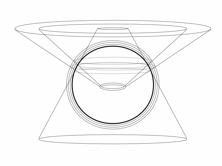
../_images/cones.svg — Geometry of a given latitude on the Earth¶

So the complete geometry of the local model, built with the auxiliary program atmloc2011.f, is made of:

a main series of layers made from the part of the atmospheric shells between the two cones (this is the part where the scoring takes place),
two series of side layers made from the part of the atmospheric shells between one of the two cones and the third one. These additional layers are needed to take into account the primary and secondary particles which don’t come from the vertical direction but can anyway reach the region of interest.

Atmospheric model: density¶

The atmosphere can be roughly characterized as the region from sea level to about 1000 km altitude around the globe, where neutral gases can be detected. Below 50 km the atmosphere can be assumed to be homogeneously mixed and can be treated as a perfect gas. Above 80 km the hydrostatic equilibrium gradually breaks down as diffusion and vertical transport become important.

Table 16.1 shows the U.S. Standard Atmosphere depth vs. altitude and vs. FLUKA atmospheric layer.

Number of region related to the atmospheric layer in FLUKA, altitude in km of the lower radius of the atmospheric layer, U.S. Standard Atmosphere depth in $g/cm^{2}$.¶
	km	US St.		km	US St.		km	US St.
FLUKA	from	Atm.	FLUKA	from	Atm.	FLUKA	from	Atm.
region	s.l.	Depth	region	s.l.	Depth	region	s.l.	Depth
		(g/cm$^2$)			(g/cm$^2$)			(g/cm$^2$)
1.0	70.0	0.092	35.0	31.6	9.367	69.0	10.7	242.777
2.0	68.5	0.108	36.0	30.8	10.540	70.0	10.2	260.107
3.0	67.1	0.126	37.0	30.0	11.849	71.0	9.8	278.093
4.0	65.6	0.146	38.0	29.2	13.309	72.0	9.4	296.729
5.0	64.2	0.170	39.0	28.4	14.937	73.0	8.9	316.007
6.0	62.8	0.198	40.0	27.7	16.748	74.0	8.5	335.921
7.0	61.5	0.230	41.0	26.9	18.763	75.0	8.1	356.460
8.0	60.1	0.266	42.0	26.2	21.004	76.0	7.7	377.615
9.0	58.8	0.308	43.0	25.5	23.492	77.0	7.3	399.374
10.0	57.5	0.356	44.0	24.8	26.255	78.0	6.9	421.727
11.0	56.2	0.411	45.0	24.1	29.290	79.0	6.6	444.661
12.0	55.0	0.474	46.0	23.4	32.613	80.0	6.2	468.163
13.0	53.8	0.546	47.0	22.7	36.244	81.0	5.8	492.219
14.0	52.5	0.628	48.0	22.1	40.205	82.0	5.5	516.815
15.0	51.4	0.722	49.0	21.4	44.516	83.0	5.1	541.936
16.0	50.2	0.828	50.0	20.8	49.201	84.0	4.8	567.566
17.0	49.1	0.950	51.0	20.2	54.283	85.0	4.4	593.691
18.0	47.9	1.088	52.0	19.6	59.785	86.0	4.1	620.295
19.0	46.8	1.245	53.0	19.0	65.733	87.0	3.8	647.359
20.0	45.7	1.423	54.0	18.4	72.152	88.0	3.4	674.869
21.0	44.7	1.625	55.0	17.8	79.068	89.0	3.1	702.807
22.0	43.6	1.854	56.0	17.2	86.506	90.0	2.8	731.155
23.0	42.6	2.112	57.0	16.7	94.493	91.0	2.5	759.898
24.0	41.6	2.404	58.0	16.1	103.057	92.0	2.2	789.016
25.0	40.6	2.734	59.0	15.6	112.224	93.0	1.9	818.493
26.0	39.6	3.106	60.0	15.0	122.023	94.0	1.6	848.311
27.0	38.7	3.525	61.0	14.5	132.482	95.0	1.3	878.453
28.0	37.7	3.996	62.0	14.0	143.628	96.0	1.1	908.900
29.0	36.8	4.526	63.0	13.5	155.489	97.0	0.8	939.636
30.0	35.9	5.121	64.0	13.0	168.094	98.0	0.5	970.643
31.0	35.0	5.789	65.0	12.5	181.471	99.0	0.3	1001.903
32.0	34.1	6.538	66.0	12.0	195.646	100.0	0.0	1033.400
33.0	33.3	7.378	67.0	11.6	210.649
34.0	32.4	8.317	68.0	11.1	226.507

Geomagnetic field¶

In the last 50 years measurements of the geomagnetic field configuration have been performed regularly with increasing precision, revealing a yearly weakening of the field intensity of 0.07% and a westward drift of $\approx 0.2$ degrees per year over the Earth ’s surface.

This field can be described, to first order, as a magnetic dipole tilted with respect to the rotation axis by $\approx 11.5^\circ$, displaced by $\approx 400$ km with respect to the Earth’s center and with a magnetic moment $M = 8.1 \times 10^{25}$ G cm$^3$. The dipole orientation is such that the magnetic South pole is located near the geographic North pole, in the Greenland, at a latitude of $75^\circ$ N and a longitude of $291^\circ$. The magnetic North pole is instead near the geographic South pole, on the border of the Antarctica. The intensity at the Earth’s surface varies from a maximum of $\approx 0.6$ G near the magnetic poles to a minimum of $\approx 0.2$ G in the region of the South Atlantic Anomaly (SAA), between Brazil and South Africa. The complex behavior of the equipotential field lines is mainly a consequence of the offset and tilt.

In FLUKA the geomagnetic field is taken into account in two different stages of the simulation chain.

Effect of geomagnetic cutoff which modulates the primary spectrum: at a given location (point of first interaction of primary particles) and for a given direction a threshold in magnetic rigidity exists. The closer the injection point is to the geomagnetic equator, the higher will be the vertical rigidity threshold. The standard possibility offered to the user is to evaluate the geomagnetic cutoff making use of a dipolar field centered with respect to the centre of the Earth, adapted to give the “correct” vertical rigidity cutoff for the geographic location under examination.

Under this approximation, an analytical calculation of the cutoff can be performed and the FLUKA source routine for galactic cosmic rays can apply the resulting geomagnetic cutoff. In case an off-set dipole (not provided at present) or more sophisticated approaches are deemed necessary, a spherical harmonic expansion model like the IGRF model is available [CLIMAX]. However no default mean is provided for making use of these higher order approximations for computing geomagnetic cutoff’s, since no analytical calculation is possible, and a numerical (back)tracking of the primary particle from(/to) infinity is required.

Please note that activating these more realistic options for the earth geomagnetic field by means of the GCR–SPE card has only the effect of using the resulting field while showering in the atmosphere (see next point), a minimal correction with respect to the dominant effect of the geomagnetic cutoff.
The local geomagnetic field can be taken into account during shower development in the atmosphere. The field is automatically provided by the default MAGFLD FLUKA user routine, in accordance to the option selected in the GCR–SPE card. For local problems, provided the coordinate system is consistently used (that is, geomagnetic coordinates for the dipolar field, geographic ones for the multipolar field) there is no need to provide any orientation or intensity information about the field.

Scoring¶

The usual scoring options (USRBDX, USRYIELD…) can be used to define detectors to calculate the fluence of different radiation fields.

The various `SDUM` options available with command `SPECSOUR`¶

For ``SDUM = GCR–ALLF``: All-nucleon flux

All-nucleon flux as explained in The High Energy All-Nucleon Spectrum. Three different options (average, maximum and minimum flux) are available. The program reads fluxes from a file named allnucok.dat in which are given the total energy (GeV), the fluxes ($E \times dN/dE$) and the neutron/proton ratios. It is possible to give an energy interval and to choose a starting radius (radius of the emission sphere in case of spherical geometry) or starting height (the emission height in case of flat geometry). It is possible to activate the vertical geomagnetic cutoff and to give the cutoff value at the central latitude, otherwise the geomagnetic cutoff will be not taken into account. Ions are treated like separate nucleons, or as alphas and protons.

WHAT(1) = 1.0:: central value
= 2.0:: minimum value
= 3.0:: maximum value
WHAT(2) ≥ 0.0:: starting radius (cm)
< 0.0:: starting height (cm)
WHAT(3) =: Minimum energy
WHAT(4) =: Maximum energy
WHAT(5) =: Spectral index for sampling (below transition energy)
WHAT(6) =: Transition energy for sampling (above it, sample from $1/E$)
SDUM: : not used

Continuation card:

WHAT(1) = 0.0:: no geomagnetic cutoff
= 1.0:: geomagnetic cutoff is requested
= 2.0:: the vertical geomagnetic cutoff is read as WHAT(2)
WHAT(2) =: vertical geomagnetic cutoff at central latitude for WHAT(1) = 2.0, no meaning otherwise
WHAT(3): – WHAT(5): no meaning
WHAT(6) ≤ 0.0:: nucleons are transported separately
> 0.0:: transport as many $\alpha$s as can be built by neutrons, and the remaining protons
SDUM: = “ & ” in any position in column 71 to 78 (or in the last field if free format is used)

For ``SDUM = GCR–AMS``: AMS All-particle flux

All-particle flux (ion flux), as explained in The AMS All-Particle Spectrum. The particle composition of the flux can be modified by choosing the minimum and maximum atomic number (1 ≤ Z ≤ 28). The spectrum components have been produced applying the solar modulation with the modified Badhwar code for various modulation parameters to the LIS spectra based on AMS02 data of ref.[DTL22] and written on “.spc” files (Z+<PhiMV>+.spc). It is possible to give an energy interval and to choose a starting radius (radius of the emission sphere in case of spherical geometry) or starting height (the emission height in case of flat geometry). It is possible to activate the geomagnetic cutoff (WHAT(7) in SPECSOUR) and to input optionally the vertical cutoff value at the central latitude.

Ions are treated like real ions or can be splitted. The optimized value for spectral index for sampling (below transition energy) is $\gamma = 1.75$ (WHAT(5)). Above transition energy, the spectrum will be assumed to have a $1/E$ shape. Proper weights are then applied to account for the actual spectral indeces. This procedure allows to sample also the high energy tails of the primary spectra. It must be noted that this is a form of source spectrum biasing and therefore no analogue runs are possible.

For SDUM = GCR-GSF: GSF All-particle flux¶

All-particle flux (ion flux), as explained in The GSF All-Particle Spectrum. The same considerations as for GCR-AMS apply. The particle composition of the flux can be modified by choosing the minimum and maximum atomic number (1 =< Z =< 28). The spectrum components have been produced applying the solar modulation with the modified Badhwar code [Bad96] for various modulation parameters to the LIS spectra based on Global SPline Fit data of ref. [Hpd17] and written on ’.spc’ files (Z+A+<GsfMV>+.spc). It is possible to give an energy interval and to choose a starting radius (radius of the emission sphere in case of spherical geometry) or starting height (the emission height in case of flat geometry). It is possible to activate the geomagnetic cutoff (WHAT(7) in SPECSOUR) and to input optionally the vertical cutoff value at the central latitude. Ions are treated like real ions or can be split. The optimized value for spectral index for sampling (below transition energy) is gamma = 1.75 (WHAT(5)). Above transition energy, the spectrum will be assumed to have a 1/E shape. Proper weights are then applied to account for the actual spectral indeces. This procedure allows to sample also the high energy tails of the primary spectra. It must be noted that this is a form of source spectrum biasing and therefore no analogue runs are possible.

For ``SDUM = GCR–IONF``: All-particle flux

All-particle flux (ion flux), as explained in The OLD All-Particle Spectrum. The particle composition of the flux can be modified by choosing the minimum and maximum atomic number (1 ≤ Z ≤ 28). The spectrum components have been produced by the modified Badhwar code for various modulation parameters and written on “.spc” files (Z+<PhiMV>+.spc). It is possible to give an energy interval and to choose a starting radius (radius of the emission sphere in case of spherical geometry) or starting height (the emission height in case of flat geometry). It is possible to activate the geomagnetic cutoff (WHAT(7) in SPECSOUR) and to input optionally the vertical cutoff value at the central latitude.

For ``SDUM = SPE–SPEC, SPE–2003 or SPE–2005``: the source is a Solar Particle Event

The input parameters are the same for the three SDUM values.
For SDUM = SPE–SPEC or SPE–2005, the spectrum is read from a file sep20jan2005.spc.
For SDUM = SPE–2003, the spectrum is read from a file sep28oct2003.spc.

WHAT(1) =: $Z_{max} + 100 \times Z_{min}$ ($Z_{min} = 1$ if none is defined)
WHAT(2) =: Starting radius (cm)
WHAT(3) =: Minimum energy
WHAT(4) =: Maximum energy

If maximum and minimum energy differ by less than 5% then a fixed energy (= Maximum energy) is sampled
WHAT(5) =: Spectral index for sampling (below transition energy)
WHAT(6) =: Transition energy for sampling (above it, sample from $1/E$)
SDUM: : not used